DataBase (3-1)

dlwogns·2023년 4월 4일

3-1

목록 보기

3/3

Relational Database

관계형 데이터베이스는 table의 모임으로 구성되어 있다.
행 -> tuple 열 -> attribute(or columns)

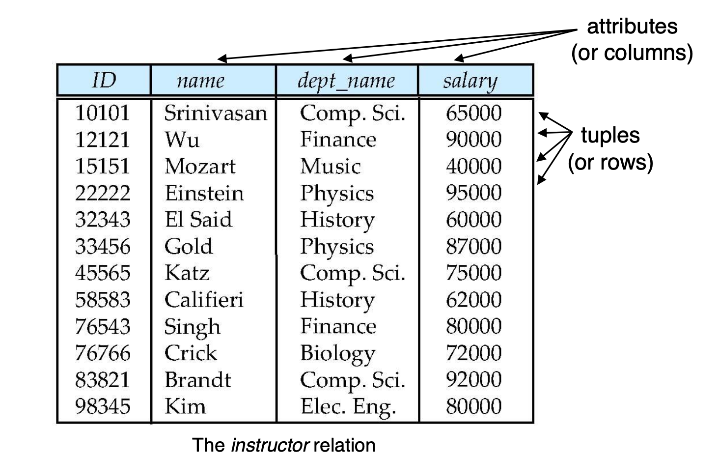
A1, A2, ..., An -> attributes

D1, D2, ..., Dn -> domains of attributes
attribute에 할당된 속성의 값, 타입, 제한사항의 범위를 나타냄.
attribute의 domain은 atomic하다, 즉 나눌 수 없다.
특별한 값인 null은 모든 domain의 요소이다..

relation은 D1 D2 Dn의 부분집합이다.
그러므로, relation은 n-tuple(a1, a2, an)의 집합이다.
-> n-ary relation이라고 하기도 함.(n-double, n-triple~~)

relation -> a table that contains rows and columns.
domain -> set of possible values that can be assigned to a particular attribute in a relation.

Database schema -> datbase의 논리적 디자인.
Database Instance -> A snapshot of the data in the database at a given instant in time

bad design

중복된 데이터 들어감.
불필요한 null 들어감.(공백이 생김)

attribute A1, A2, ..., An이 주어졌을떄, relation schema는 r (A1, A2, ..., An )를 의미한다.(e.g., instructor (ID, name, dept_name, salary))-> 이 문법은 꼭 기억해두기.r (A1, A2, ..., An )
relation schema -> a relation schema refers to the structure of a table, including the names of its columns and the data types of the values in each column.

relation instance -> A relation instance, on the other hand, refers to a specific set of rows (records) and columns (attributes) that exist in a table at a given moment in time. Each row in a relation instance represents a single record or entity, and each column represents a specific attribute or property of that entit

Relations are not ordered

Order of tuples does not matter.
Tuples may be stored in an arbitrary order

Keys

Attribute 전체의 집합 -> R

super key

만약 K가 relation에서 특정한 tuple을 나타내기에 충분하다면 , 이를 R의 superkey 라고 한다.
Example: {ID} and {ID, name} are both superkeys of instructor.

A,B,C,D arrtibutes가 있다고 했을때, super key가 A,B,C라면
A B C 가 완벽하게 같은 tuple은 없어야 한다.
database는 duplicate하지 않다고 항상 가정하기 때문에, 모든 attribute의 집합이 super가 될 수 있음.
그중에서 가장 적은 개수로, 나타낼 수 있다면, 그것을 candidate key라고 함.
-> 모든 candidate key 는 super key이지만, 모든 super key는 candidate key가 아님.

candidate key

candidate key는 superkey K의 부분집합으로, 그 중에서 오직 각각의 값이 하나씩만 가지고 있는 키들의 집합을 의미한다.
Example: {ID} is a candidate key for Instructor

primary key

candidate keys 중 하나가 primary key로 지정된다.

foreign key

어떤 relation이 다른 relation을 참조하는 경우,
foreign key는 어떤 테이블의 column의 집합으로, 다른 테이블의 primary key를 인용한 키 들을 의미한다.

foreign key constraint

The foreign key constraint ensures that any value in the foreign key column of the referencing table must match a value in the primary key column of the referenced table, or be null.
-> foreign key를 사용한다면, 이것을 인용한 테이블과 값이 전부 같아야 한다. 또는 null이 사용되어야 한다고 한다. -> Null은 확인해야됨.

SQL

Create

create table r(A1 D1, A2 D2, ~ An Dn)

create table instructor(
	ID		char(5),
    name	varchar(20) not null,
    dept_name varchar(20),
    salary	numeric(8,2)
)

insert into instructor values ('10211', 'Smith', 'Biology', 66000);

Integrity Constraints

primary key(A1, ~~, An)
foreign key(Am, ~~, An) references r
not null

create table instructor(
	ID		char(5),
    name	varchar(20) not null,
    dept_name varchar(20),
    salary	numeric(8,2),
    primary key(ID),
    foreign key(dept_name) references department
)


create table student(
	ID varchar(5) primary key,
    -- 이렇게 써줄 수 도 있다.
)

Alter

alter table r add A D
-> relation에서의 tuple들은 새로운 attribute에 대한 값이 null로 저장된다.
alter table r drop A

Select

select A1, A2~~An
from r1, r2 ~~rn
where P

P-> predicate

SQL query는 대소문자가 상관 없다.

sql allows duplicates in relations as well as in query results.

select distinct dept_name from instructor

-> distinct를 사용하면 duplicates를 제거한다.

select all dept_name from instructor

-> all을 사용하면 duplicates가 제거되지 않은 상태로 보여준다.

select * from instructor

-> * 은 모든 attributes를 의미한다.

select ID, name, salary/12 from instructor

-> select문은 arithmetic expressions를 constants나 attributes에 사용할 수 있다.
-> 위의 구문은 instructor relation과 같게 나오지만, salary만 /12가 된 상태로 나오는 것을 알 수 있다.

select name
from instructor
where dept_name = 'Comp. Sci' and salary > 80000

-> where은 결과가 가져야 할 조건을 특정한다.
-> 조건들은 and, or, not에 의해 조합될 수 있다.

select * from instructor, teaches

-> from 다음에는 relations가 온다.
-> 위와같은 경우, 두 relation의 cartesian product가 나오게 된다.

Join

Natural join은 공통된 attribute의 같은 값을 맞춘다.

select name, course_id from instructor natural join teaches;

같은 이름을 가지지만 관계가 없는 attributes를 같게 인식하는 것을 주의해야 한다.

select name, title
from instructor natural join teaches, course where teaches.course_id = course.course_id


select name, title 
from (instructor natural join teaches) join course using(course_id);

-> 이 두개처럼 쓰면 된다.

as

SQL 은 as를 사용해서 query에서 새로운 이름을 주는 것이 가능하다.

select ID, name, salary/12 as monthly_salary from instructor

String operation

일단 패스

Ordering the Display of Tuples

select distinct name
from instructor
order by name

-> order by를 사용해서 attribute를 기준으로 정렬할 수 있다.

order by name desc
order by name asc

-> asc, desc를 이용해 오름차순, 내림차순으로 정렬할 수 있다.

order by dept_name, name

-> multiple attributes로 정렬할 수 있다.

Where Clause Predicates

between

select name
from instructor
where salary between 90000 and 100000

-> 이렇게 between predicate를 사용할 수 있다.

Tuple comparison

select name, course_id
from instructor, teaches
where (instructor.ID, dept_name) = (teaches.ID, 'Biology');

-> 이렇게 tuple의 형태로 비교할 수 있다.

Set Operation

Find courses that ran in Fall 2009 or in spring 2010

(select course_id from section where sem = 'Fall' and year = 2009)
union
(select course_id from section where sem = 'spring' and year = 2010)

Find courses that ran in Fall 2009 and in Spring 2010

(select course_id from section where sem = 'Fall' and year = 2009)
intersect
(select course_id from section where sem = 'Spring' and year = 2010)

Find courses that ran in 2009 but not in Spring 2010

(select course_id from section where sem = 'Fall' and year = 2009)
except
(select course_id from section where sem = 'Spring' and year = 2010)

union -> or , intersect -> and, except -> not
-> 각각의 operations는 복제를 자동적으로 제거한다.

복제가 있는 데이터를 얻기 위해서는, 다음에 union all같은 형식으로 써주면 된다.

Null Values

tuples가 값이 존재하지 않거나, 알려지지 않은 값이 있을때 null값을 넣는다.

is null로 null value를 체크할 수 있다.

select name
from instructor
where salary is null

null과 어떠한 비교 연산자를 사용하면, 그것은 unknown을 return한다.

OR: (unknown or true) = true, (unknown or false) = unknown (unknown or unknown) = unknown
AND: (true and unknown) = unknown, (false and unknown) = false, (unknown and unknown) = unknown
NOT: (not unknown) = unknown

그렇다고 한다.
predicate P가 unknown이라면, 이것은 true로 평가된다.
하지만 where clase 에서는 false로 평가된다.

Aggregate Functions

avg -> average value
min -> minimum value
max -> maximum value
sum -> sum of values
count -> number of values

Find the average salary of instructors in the Computer Science department

select avg(salary)
from instructor
where dept_name = 'Comp. Sci.';

Find the total number of instructors who teach a course in the Spring 2010 semester

select count (distinct ID)
from teaches
where semester = 'Spring' and year = 2010;

Find the number of tuples in the course relation

select count (*)
from course;

group by

select dept_name, avg(salary) as avg_salary
from instructor
group by dept_name;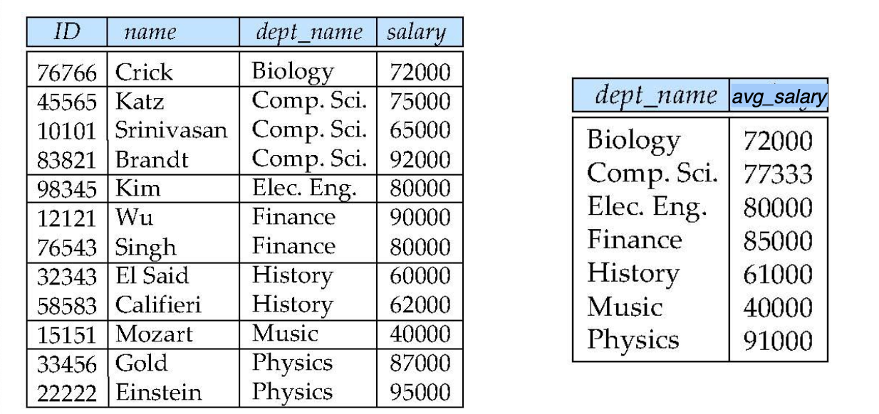

select문에 있는 attributes는 group by 다음에 항상 나와주어야 한다.

select dept_name, ID, avg(salary)
from instructor
group by dept_name;

-> 이렇게 써주면 ID때문에 에러난다.

having

where과 비슷한 역할을 하지만 having은 그룹이 만들어 진 다음에 수행이 되는 것이고, where은 그룹이 만들어 지기 이전에 수행되는 것이다.

select dept_name, avg(salary)
from instructor
group by dept_name
having avg (salary)>42000;

Null Values and Aggregate

count를 제외한 모든 aggregate operations는 null value가 있는 tuple을 무시한다.
만약 collection이 비어있다면, count는 0을 반환하고 다른것들은 null을 반환한다.

Nested Subqueries

subquery는 select-from-where 표현으로, 다른 것 안에 들어간다.

for set membership, set comparisons, set cardinality

Find courses affered in Fall 2009 and in Spring 2010

select distinct course_id
from section
where semester = 'Fall' and year = 2009 and
course_id in(select course_id from section where semester = 'Spring' and year = 2010);

Find courses affered in Fall 2009 but not in Spring 2010

select distinct course_id
from section
where semester = 'Fall' and year = 2009 and
course_id not in(select course_id from section where semester = 'Spring' and year = 2010);

Find the total number of distinct students who have taken course sections taught by the instructor with ID 10101

select count (distinct ID)
from takes
where (course_id, sec_id, semesterm year) in 
(select course_id, sec_id, semester, year
from teaches
where teaches.ID = 10101);

Set Comparison

some

Find names of instructors with salary greater than that of some (at least one) instructor in the Biology department

select distinct T.name
where instructor as T, instructor as S
where T.salary > S.salary and S.dept_name = 'Biology'

Same query using some clause

select name 
from instructor
where salary > some(select salary from instructor where dept_name = 'Biology');

some을 쓰면, 그 다음에 나오는 집합 중 어떤 원소라도 조건을 만족하면 True이다.

all

Find the names of all instructors whose salary is greater than the salary of all instructors in the Biology department

select name
from instructor
where salary > all(select salary from instructor where dept_name = 'Biology');

exists

exist 는 subquery가 nonempty라면 true를 return한다.

Find all courses taught in both the Fall 2009 semester and in the Spring 2010 semester

select course_id
from section as S
where semester = 'Fall' and semester = 2009 and 
exist(select * from section as T where semester = 'Spring' and year = 2010 
and S.course_id = T.course_id);

Not exists

select distinct S.ID, S.name
from student as S
where not exists ( (select course_id
from course
where dept_name = ’Biology’) except
(select T.course_id from takes as T where S.ID = T.ID));

-> 이게 뭐지

unique

-> 대부분의 DB에서 구현이 안되있음.

Derived Relations

subquery를 from 문에서도 쓸 수 있음.

select dept_name, avg_salary
from( select dept_name, avg(salary) as avg_salary
	from instructor
    group by dept_name)
   where avg_salary > 42000;

-> 이렇게 쓰면 having을 안써도 된다.

select dept_name, avg_salary
from (select dept_name, avg(salary)
	from instructor
    group by dept_name) as dept_avg(dept_name, avg_salary)
   where avg_salary > 42000;

lateral

-> 얘도 구현 잘 안되있음.
-> 일단 unique랑 lateral은 넘어가자~

with

with을 사용해서 임시 데이터베이스를 생성해서 사용할 수 있음. 매크로처럼.

with max_budget(value) as (select max(budget)
							from department)
select budget
from department, max_budget
where department.budget = max_budget.value;

좀 더 복잡한건

with dept _total (dept_name, value) as (select dept_name, sum(salary)
from instructor
group by dept_name), dept_total_avg(value) as
(select avg(value)
from dept_total)
select dept_name
from dept_total, dept_total_avg
where dept_total.value >= dept_total_avg.value;

이런거.

Modification of the Database

Deletion

delete all instructors

delete from instructor;

delete all instructors from the Finance department

delete from instructor
where dept_name = 'Finance'

delete all tuples in the instructor relation for those instructors associated with a department located in the Watson building.

delete from instructor
where dept_name in (select dept_name from department where building = 'Watson');

Insert

insert into course
values (’CS-437’, ’Database Systems’, ’Comp. Sci.’, 4);

insert into course (course_id, title, dept_name, credits) values (’CS-437’, ’Database Systems’, ’Comp. Sci.’, 4);

두개 똑같음.

Intermediate SQL

Join

join 은 기본적으로 cartesian product이다.
그 중 두개의 relation의 tuple이 같은 값을 요한다.

SQL에서는 join predicate(join condition)이라고 하는 다른 형태의 join 또한 제공한다.

select name, course_id
from instructor, teaches
where instructor.ID = teaches.ID


select name, course_id
from instructor natural join teaches;

select name, course_id
from instructor join teaches on instructor.ID = teaches.ID;

-> 세번째 구문과 같이 on을 사용해줄 수 있다.

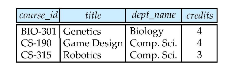
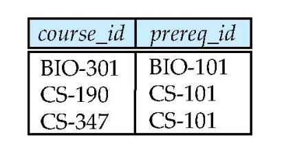
Relatioin course, prereq가 주어져 있다.
이걸 course_id로 natural join하면 값이 전부 같지 않기 때문에 cartesian product가 나오게 된다.

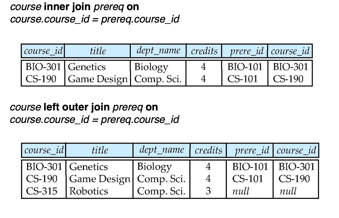
Outer Join

정보 손실을 막기위한 join의 연장선이다.
-> 보존된 tuple들은 inner join에서는 잃는다고 한다.

null value를 사용한다.

left outer Join

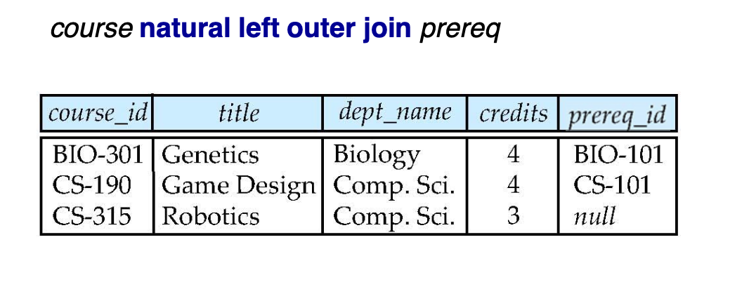
-> course의 course_id를 기준으로 한다.

Right Outer Join

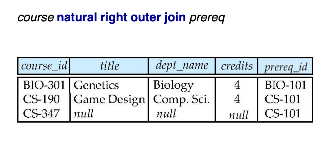
-> prereq의 course_id를 기준으로 한다.

Full Outer Join

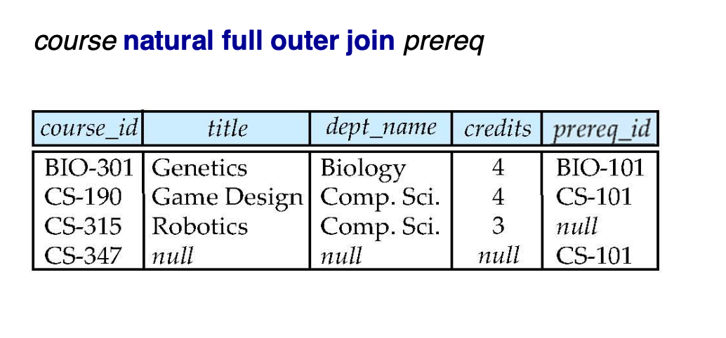
-> 두개의 값의 합집합으로 나타낸다.

join example

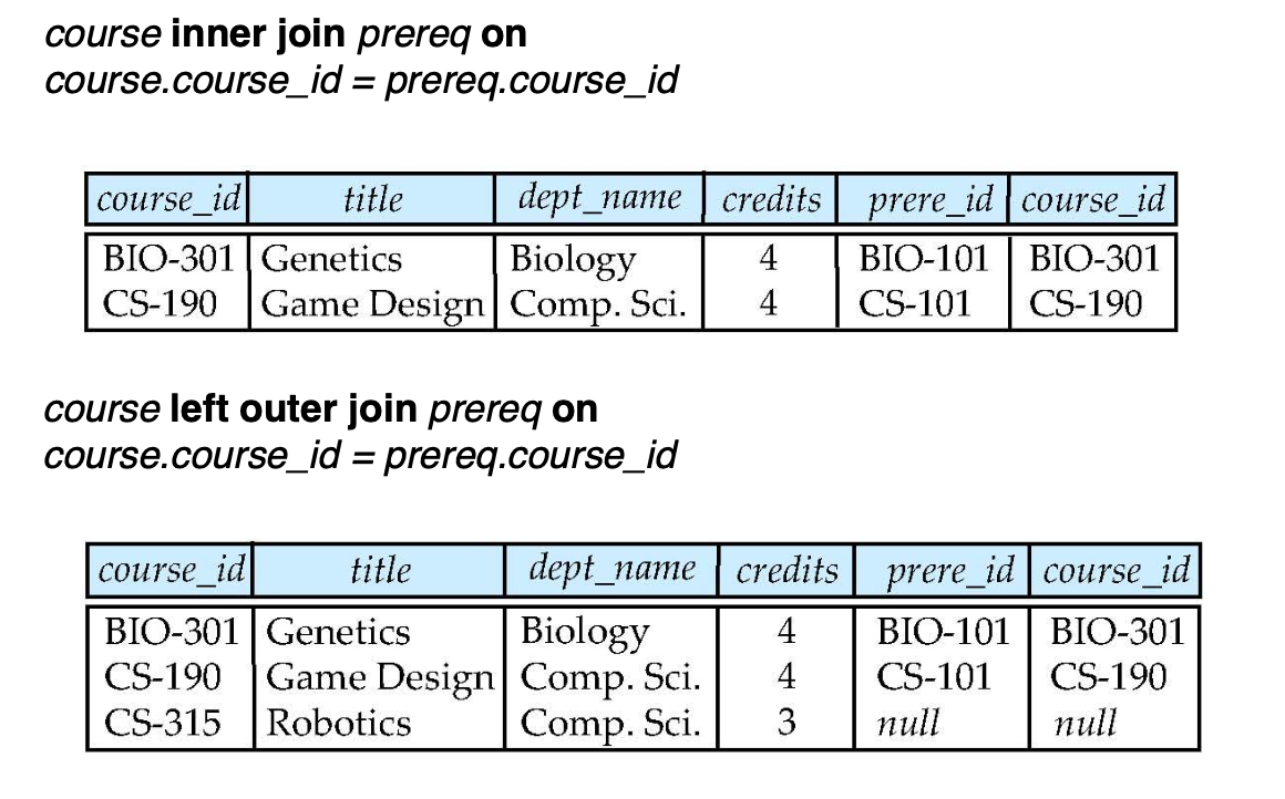
inner join하면 null이 나오게 되는 tuple은 다 버리고,

-> natural을 쓰면 겹치는 column이 사라진다.

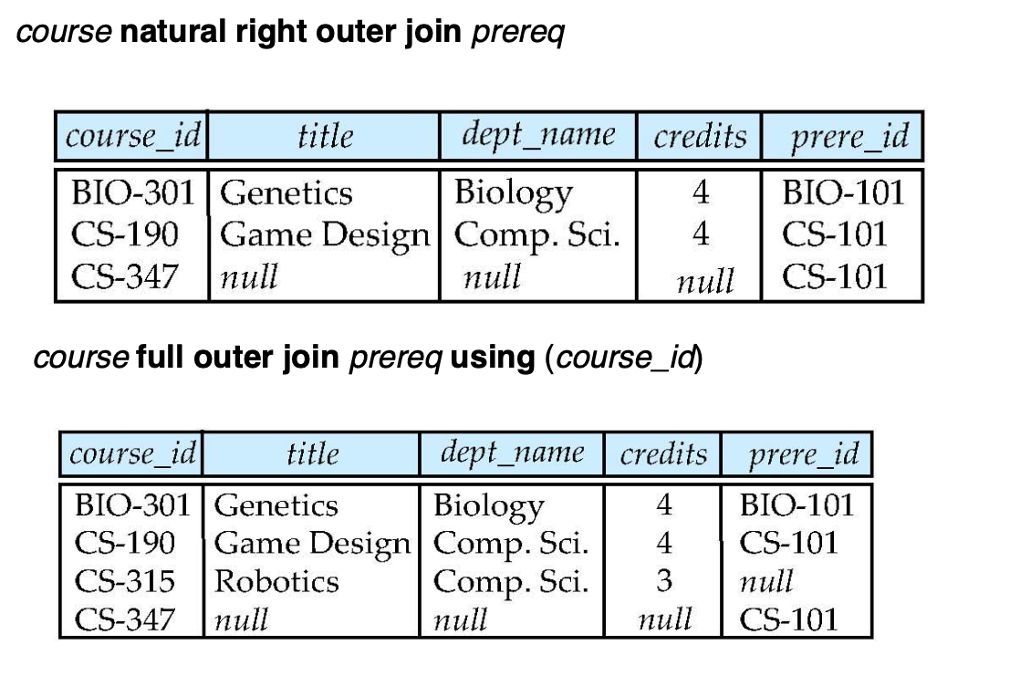
-> full outer join에 using을 사용해서 natural의 효과를 줬나?
-> 맞다. natural을 쓰면 같은 attribute 다 묶는데, using을 쓰면 using 사용한 거만 묶는다.

View

모든 사용자가 전체의 logical model을 보는 것은 좋지 않기 때문에, 특정한 사용자로 부터 특정한 데이터를 가리기 위해 쓰는 거다.
사용자에게 virtual realtion -> view

create view v as <query expression>

A view of instructors without their salary

create view faculty as
	select ID, name, dept_name
    from instructor

Find all instructors in the Biology department

select name
from faculty
where dept_name = 'Biology'

Create a view of department salary totals

create view department_total_salary(dept_name, total_salary) as 
select dept_name, sum(salary)
from instructor
group by dept_name;

Views Defined Using Other Views

create view physics_fall_2009 as
	select course.course_id, sec_id, building, room_number
    from course, section
    where course.course_id = section.course_id
    	and course.dept_name = 'Physics'
        and section.semester = 'Fall'
        and section.year = '2009';
        

create view physics_fall_2009_watson as
	select course_id, room_number
    from physics_fall_2009
    where building = 'Watson'

Update of a View

insert into faculty values('30765','Green','Music');

faculty가 instructor에서 salary빼고 만든 것 이므로
instructor relation에
('30765','Green','Music',null)
이 들어간 것이다.

Some Updates cannot be Translated Uniquely

-> 강노 17p

Constraints on a Single Relation

unique

unique(A1, A2, ~~ An)
create의 unique는 attribute A1, ~ An이 candidate key라는 것을 나타낸다. -> 이 attribute에는 중복값이 들어올 수는 없지만, null은 된다.

check

create table section (
course_id varchar (8),
sec_id varchar (8),
semester varchar (6),
year numeric (4,0),
building varchar (15),
room_number varchar (7),
time slot id varchar (4),
primary key (course_id, sec_id, semester, year),
check (semester in (’Fall’, ’Winter’, ’Spring’, ’Summer’))
);

-> semester에는 저 네개만 나올 수 있게 하는 구문.

24p부터 다시보기~

reference integrity

department relation의 primary key가 dept_name이고, instructor의 dept_name이 상단에 서술한 dept_name을 참조한 foreign key일때,instructor의 dept_name에 biology가 있다면, department의 dept_name에도 꼭 있어야 한다.

Relational DB Design

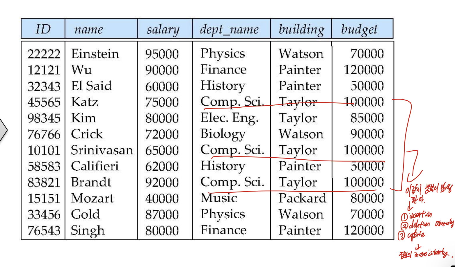
이렇게 구성하면, 밑줄친 부분에 대해서 이렇게 중복이 발생할 수 있다.

여기선 Dept_name이 building, budget을 결정한다. 하지만, deptname은 big_relation에서 candidate key가 아니다. 그렇기 때문에 중복이 발생하는 것 이다.

그러므로 이러한 FD를 잘 맞추어서 decompose 하는 것이 중요하다.

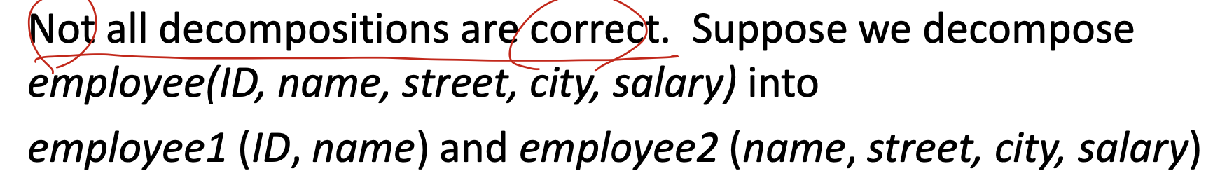
FD를 맞춰야지, 그냥 막 자르는 것도 안된다.

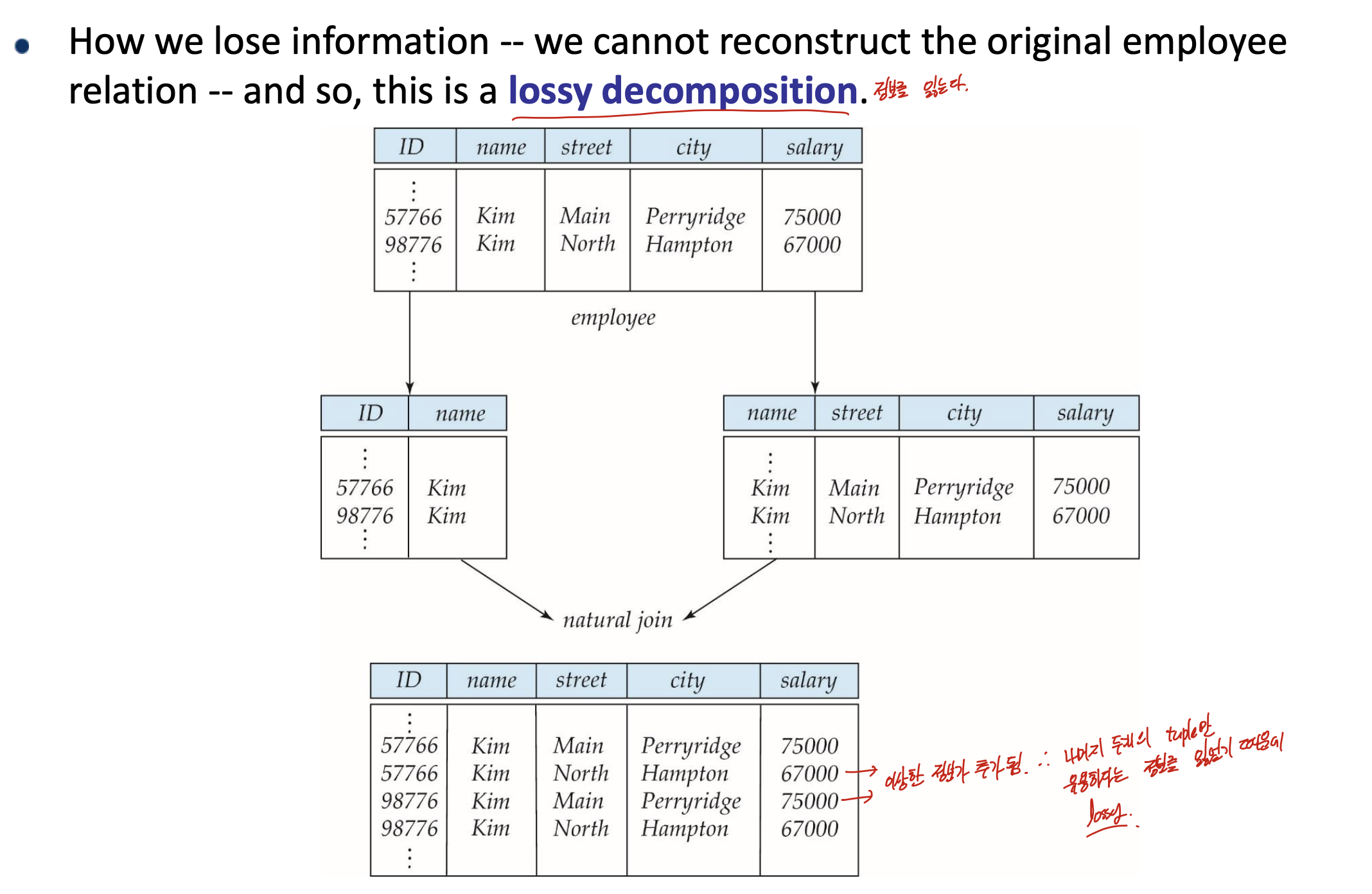
이게 그 예시인데, R을 R1, R2로 분리해서, R1 join R2의 결과가 다시 R이 나와야 된다. 하지만, 이것은 추가적인 튜플이 발생하므로서 기존 튜플이 유용하다는 정보를 잃었다. 그러므로 lossy decomposition이다.

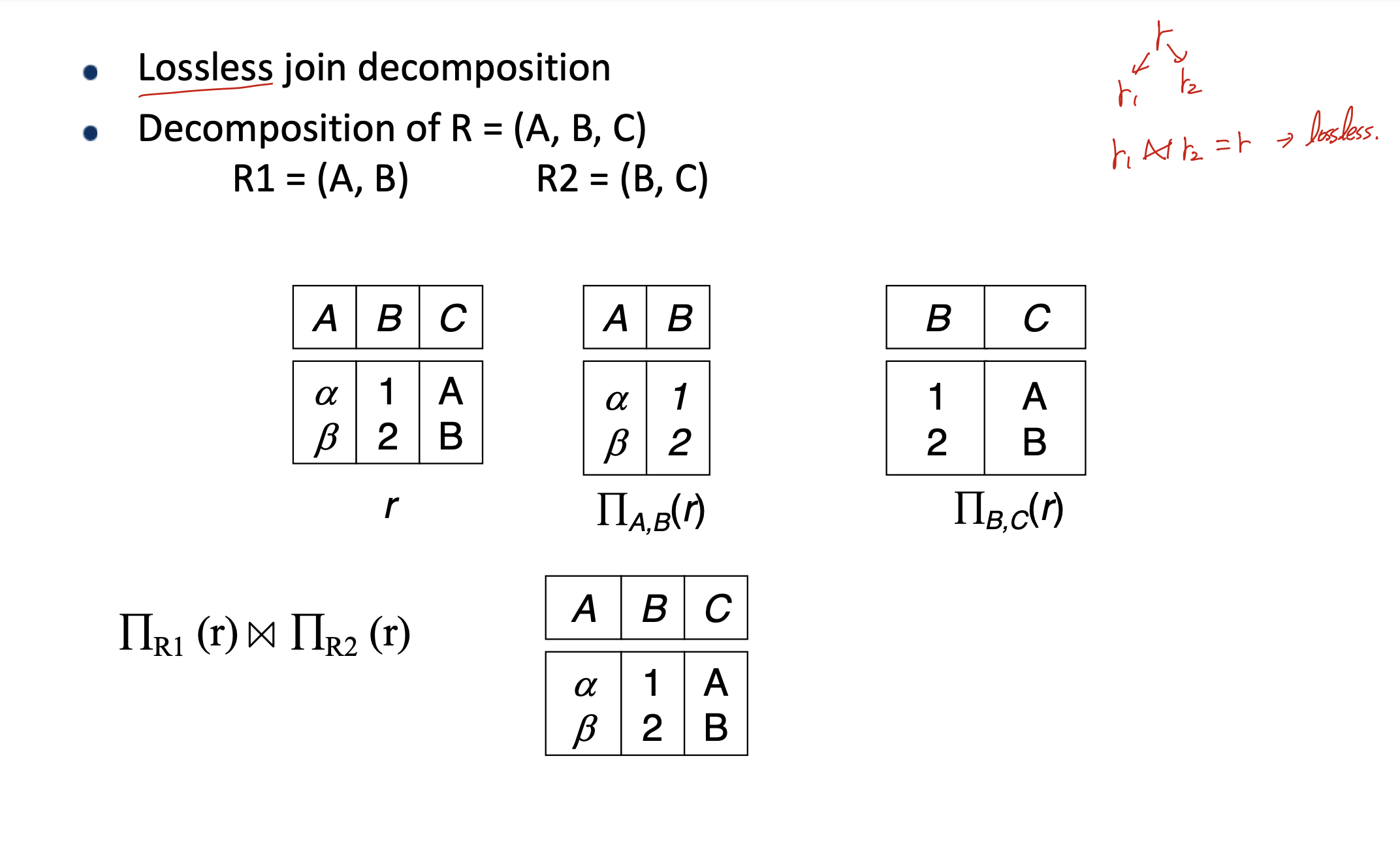
이렇게 짤라야 된다.

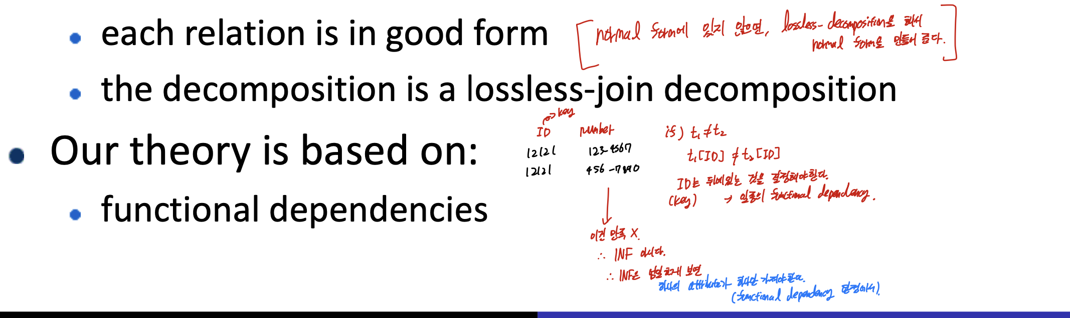
만약 기존 relation이 NF에 있지 않다면, Lossless decomposition을 사용해 normal form으로 만들어주는 것이 중요하다.
그리고 밑에 예시를 보면, 하나의 ID에 해당하는 값이 두개가 있다. 이것은 1NF가 안된다. 엄밀하게 1NF를 보면, 하나의 attribute가 하나만 가져야 된다는 특성을 가지고있다.

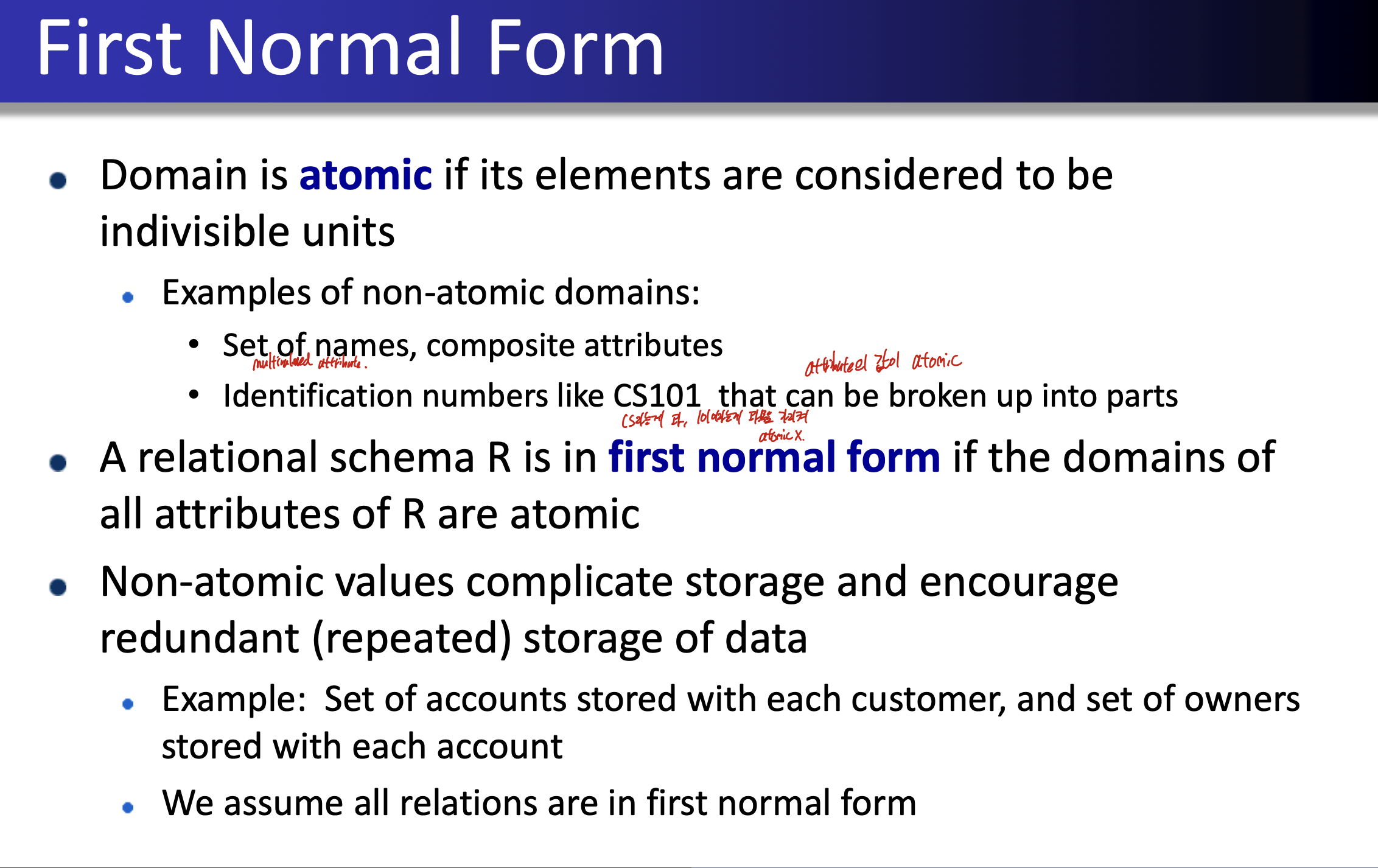
모든 Attribute의 domain이 atomic하다면, 이것은 1NF이다.
CS101 같은 예제를 보면, CS, 101을 나누어서 생각할 수 있다. 이러면 안된다.

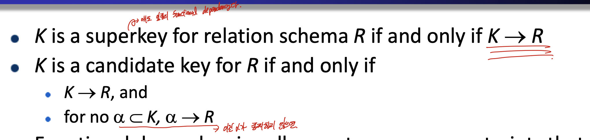
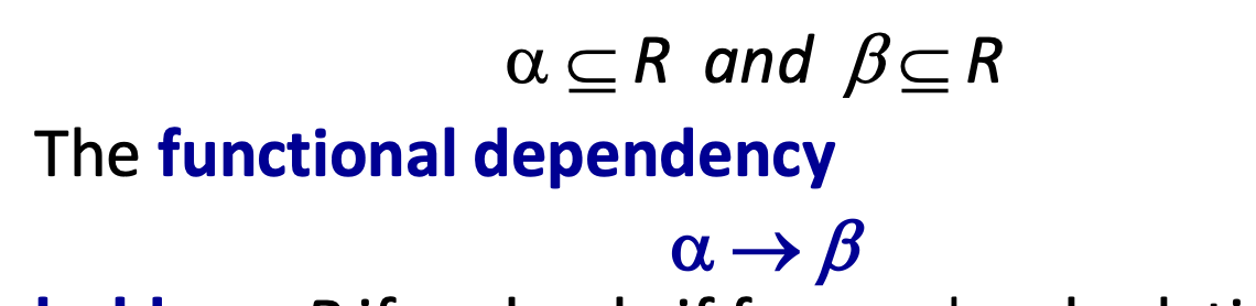
functional dependency는

key라고 생각하면 된다.
만약 K -> R이면 super key이고, a가 K에 속하고, a -> R이라면 a는 candidate key, K는 candidate key가 되지 못한다.

functional dependency는 이렇게 우연히 만족할 수 도 있다.
functional dependency는 attribute간의 관계라는 것을 알아야 한다.

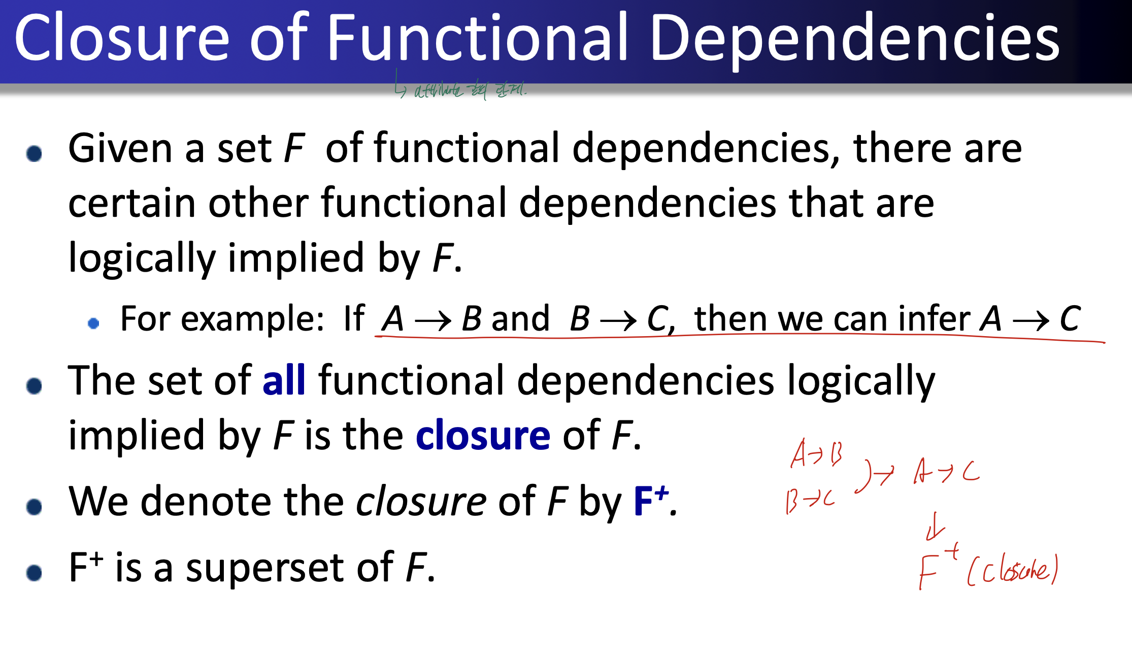
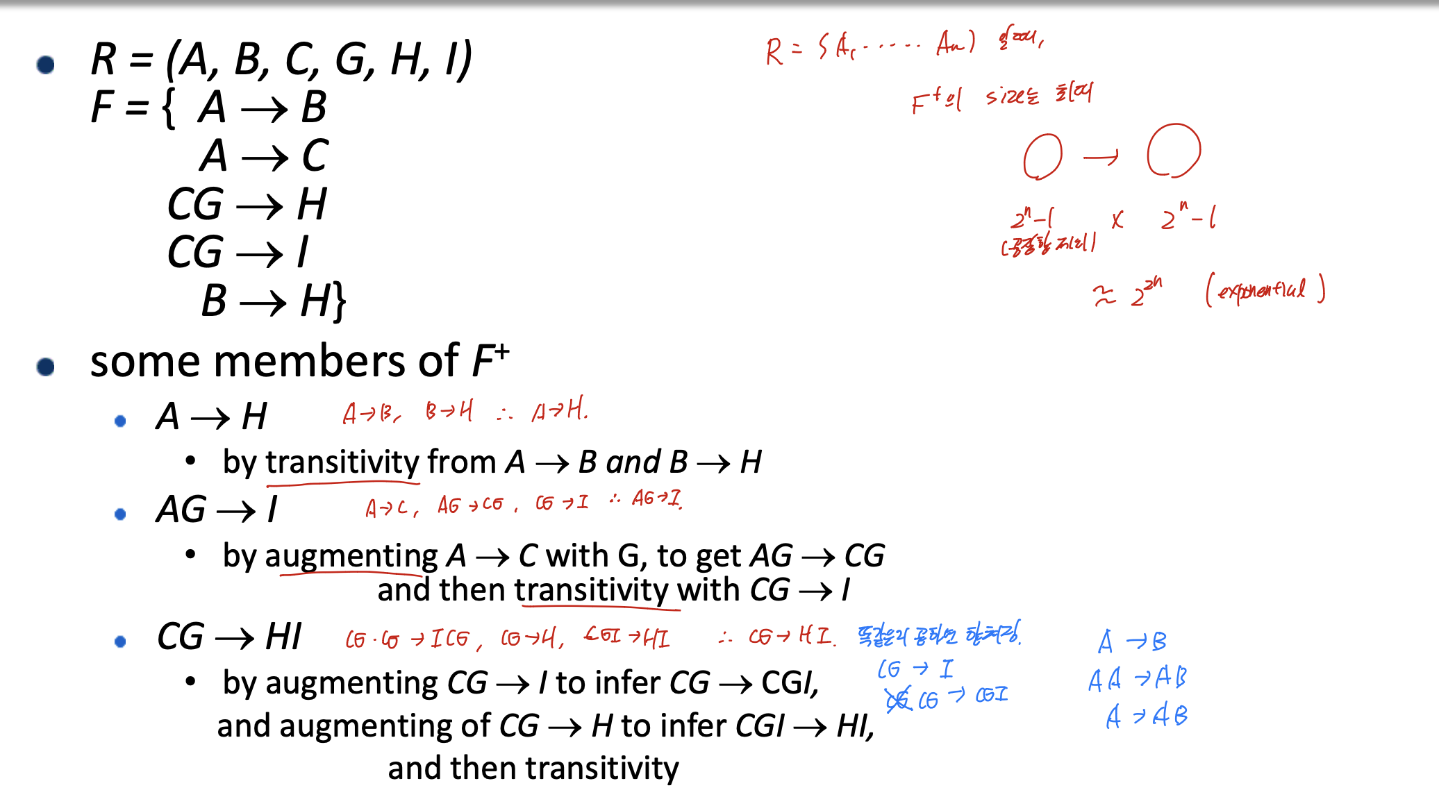
A->B, B->C일때, A->C 라는 것을 알 수 있다. 이것을 closure라고 한다.

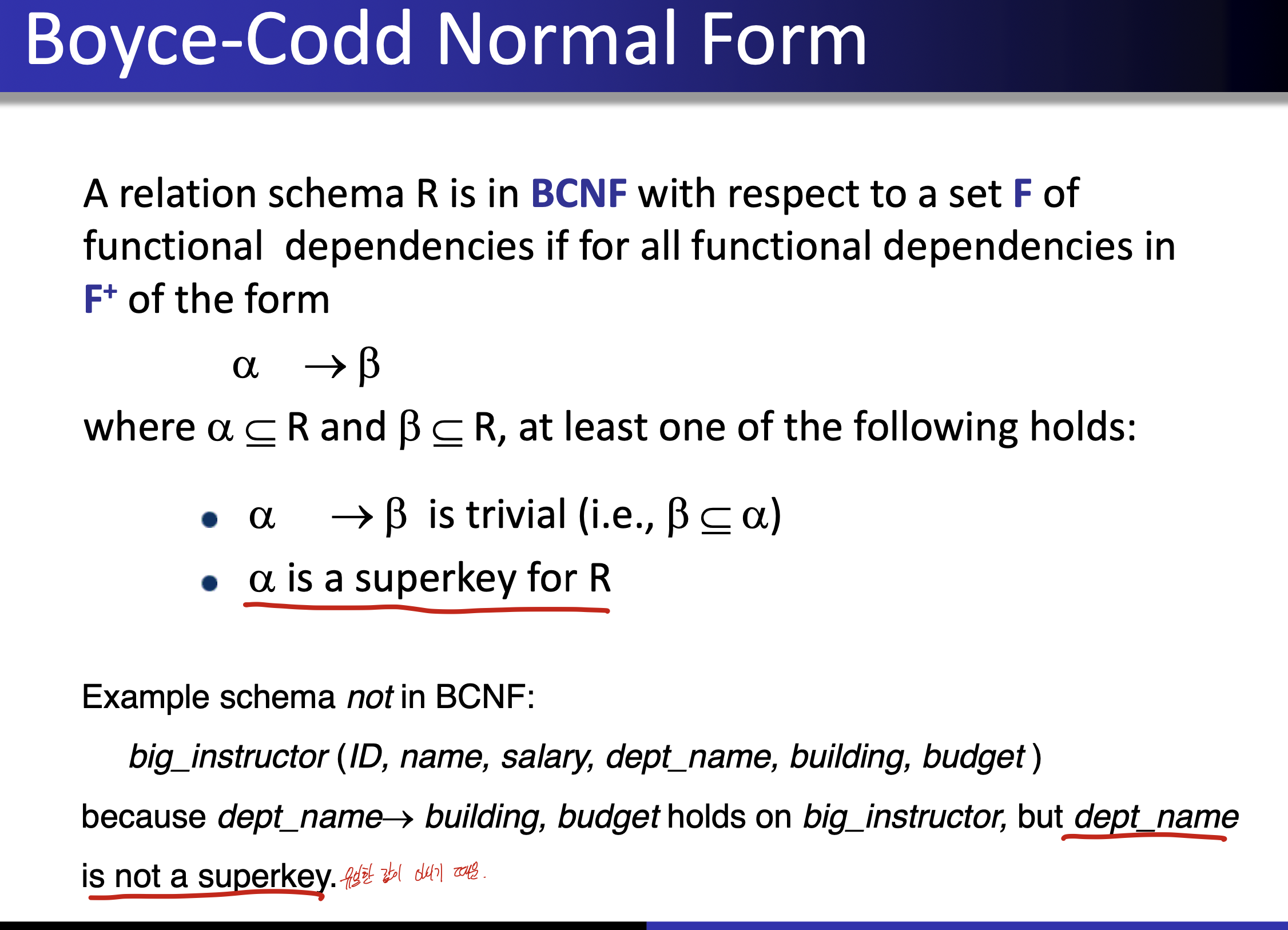
BCNF는 1NF, 2NF를 만족해야 한다.
그러므로 deptname과 같이 중복된 값이 들어간 것은 안된다.
그리고 a -> b일떄, a가 R의 superkey여야 한다.

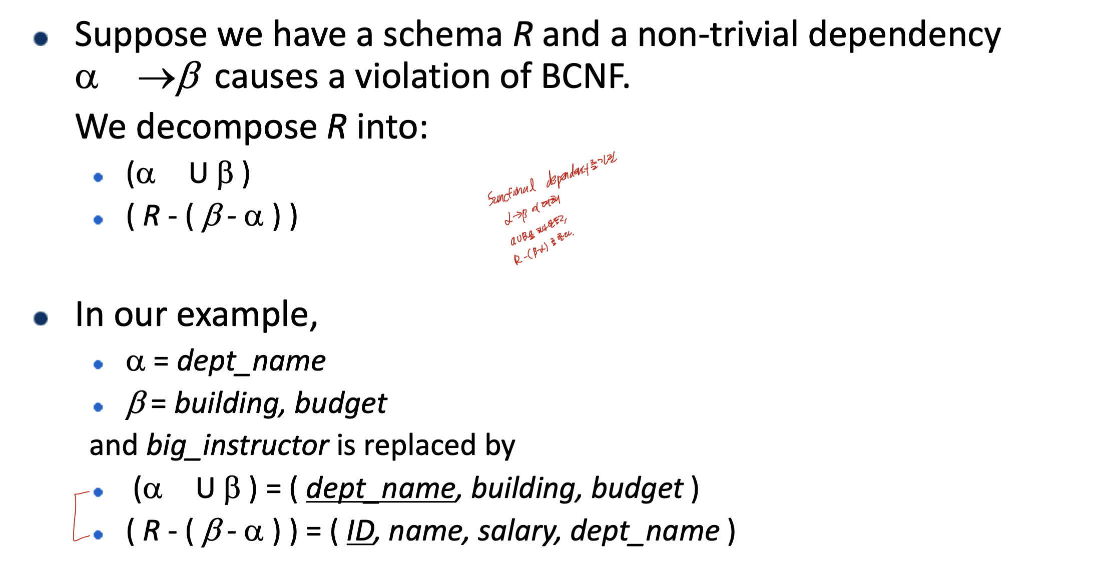
이걸 이용해서 밑의 예제와 같이 decompose할 수 있다.

R을 R1, R2로 decompose했을때, 각각의 FD가 잘 보존된다면 Dependency preserving이라 한다.
예를 들어 deptname으로 decompose한다면, 각각의 relation이 FD를 만족한다. 그러므로 Dependency preserving을 만족한다.

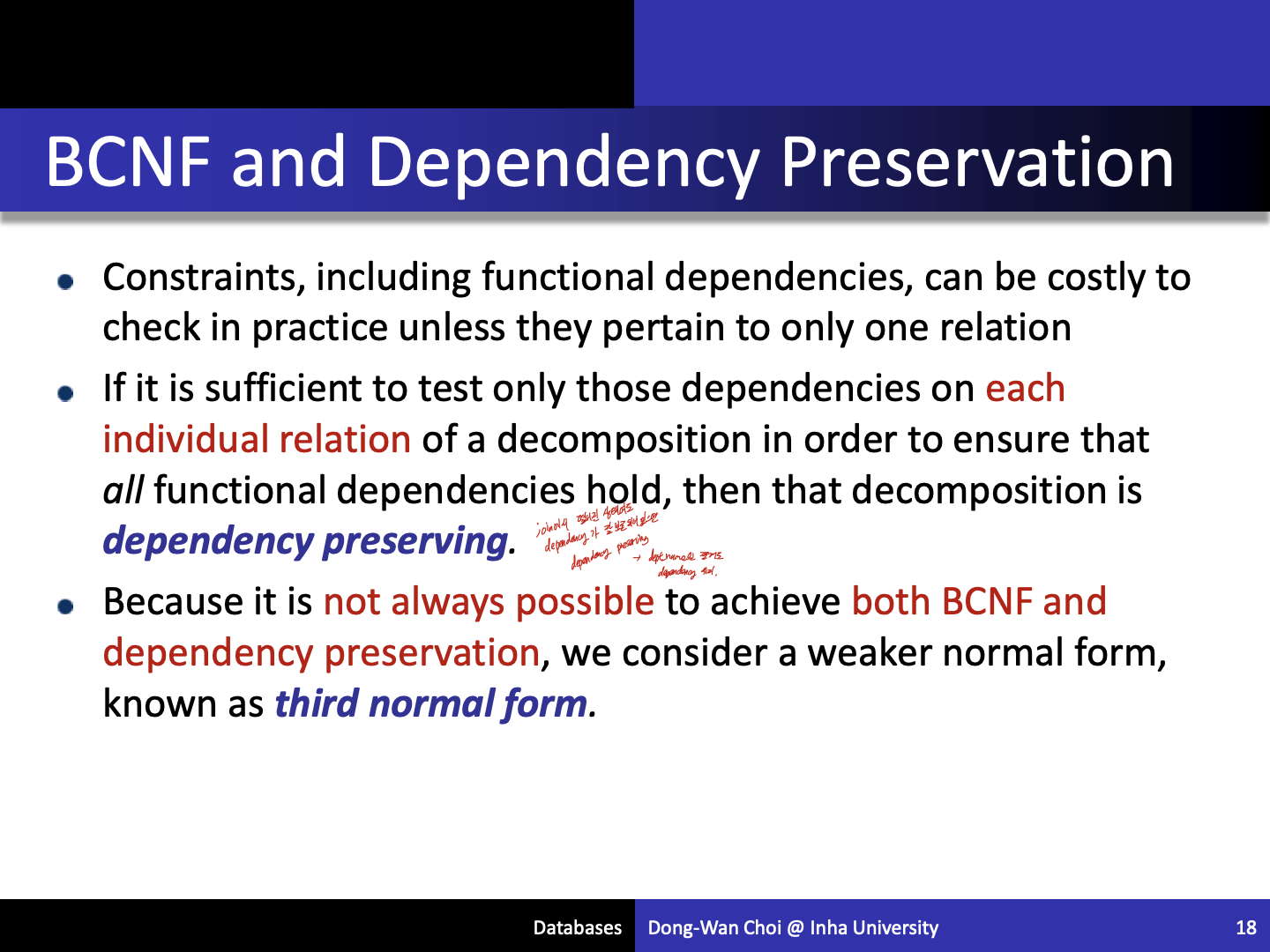
하지만 BCNF를 만족하면서 Dependency preserving을 하는 것은 항상 가능한 것은 아니다. 그러므로 조금 유해진 3NF를 고려한다.

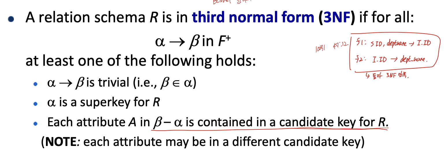
superkey 조건까지는 같다. 하지만
a->b일때, b-a의 각각의 attribute가 R의 candidate key에 포함이 된다면, 3NF이다.
a->b->c일때, a, c가 key이면 3NF 만족한다.

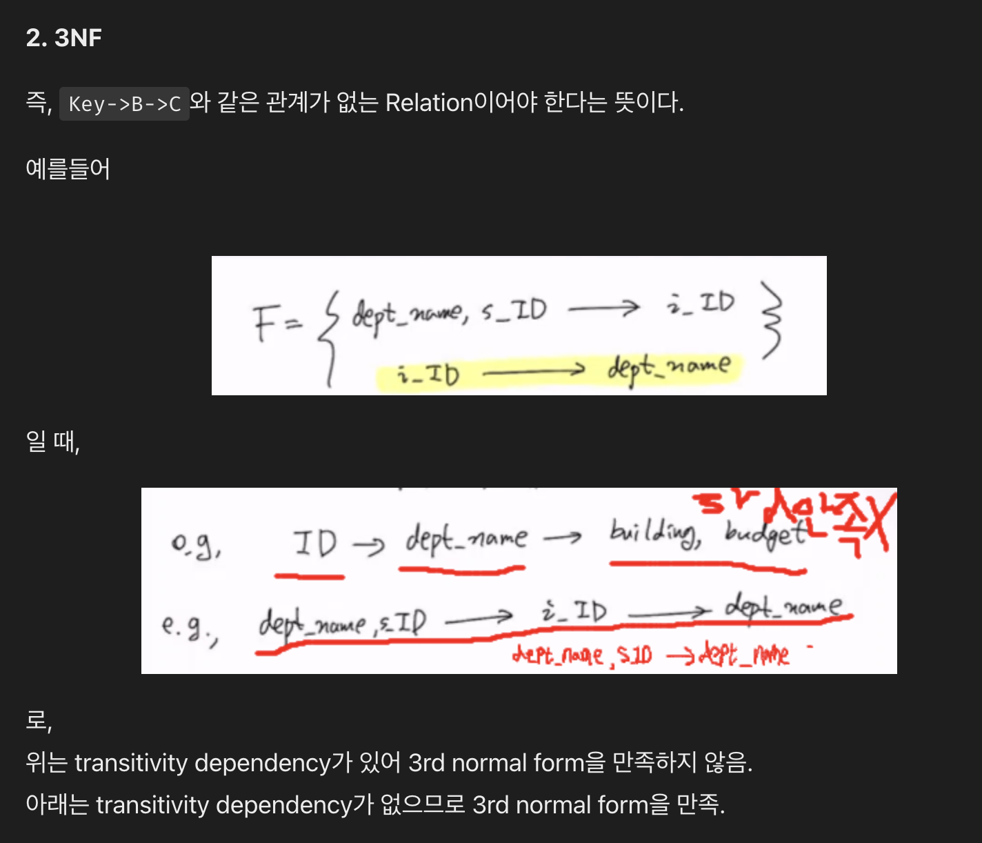
이렇게 A->B->C가 된다면 3NF를 만족하지 않는다.

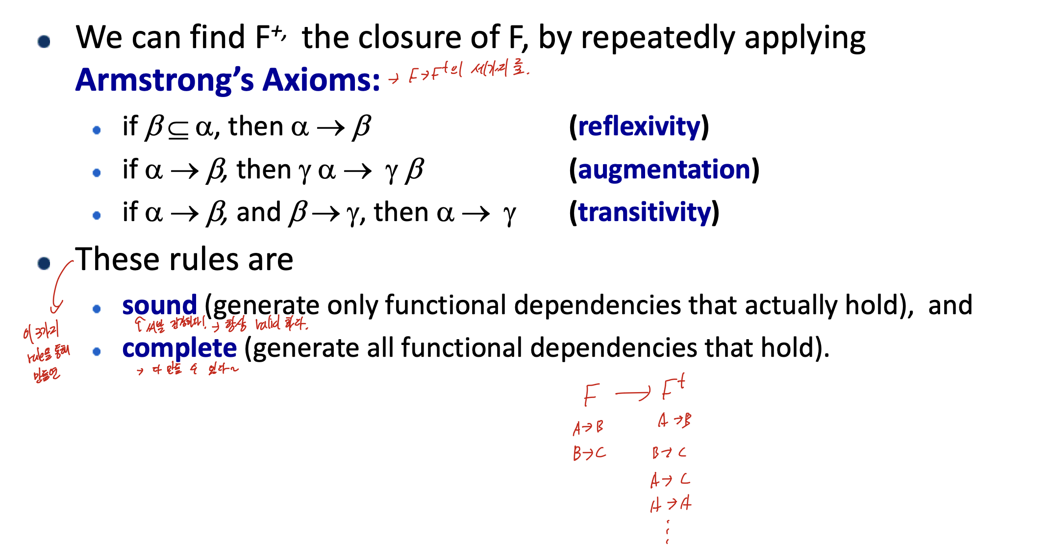
F+를 만들기 위해서는 다음 세가지 룰이 있다.

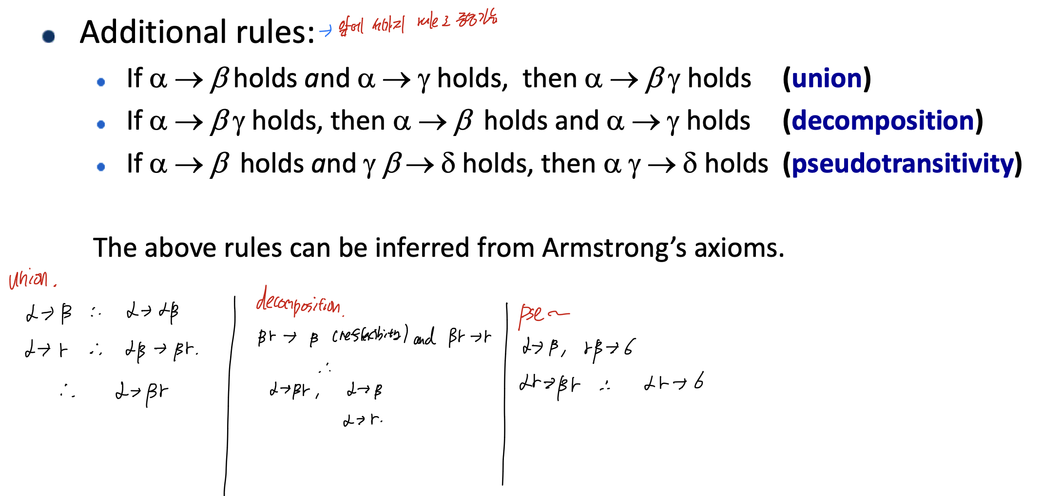
앞의 세가지의 연장선으로 세개가 더있다.

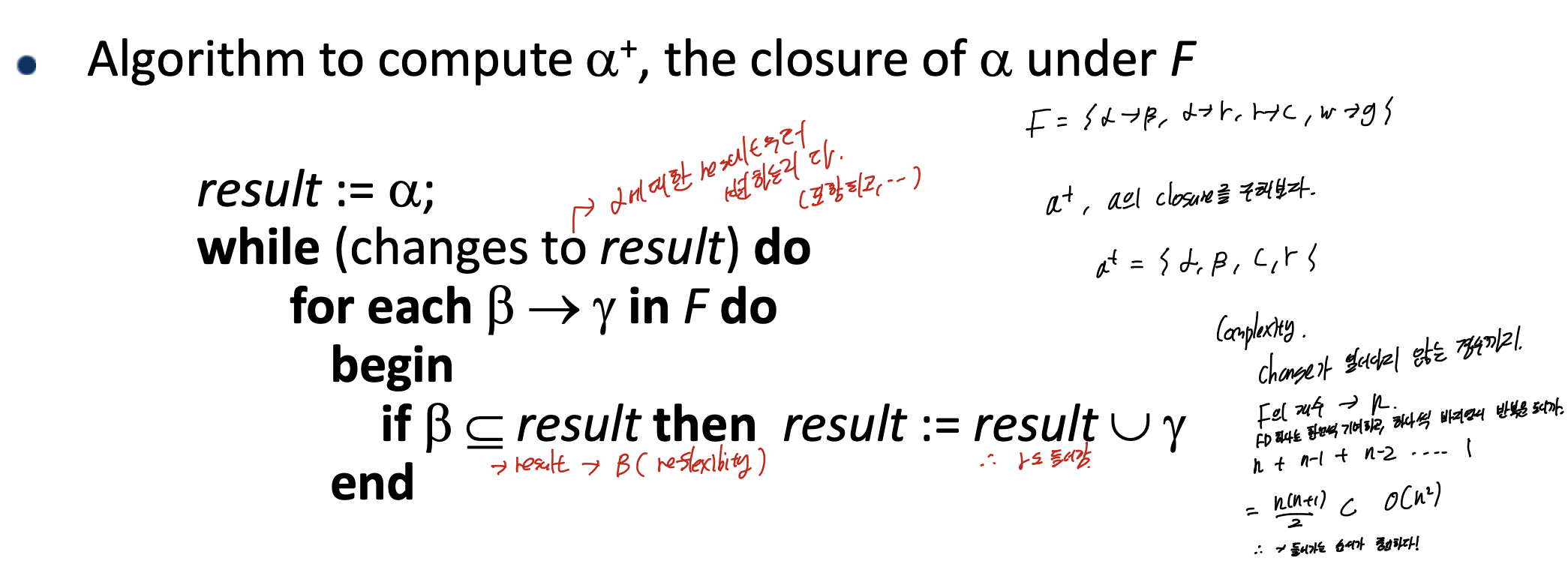
attribute의 closure이다. 이전 공식들로 구해지는것들의 전체의 집합이다.

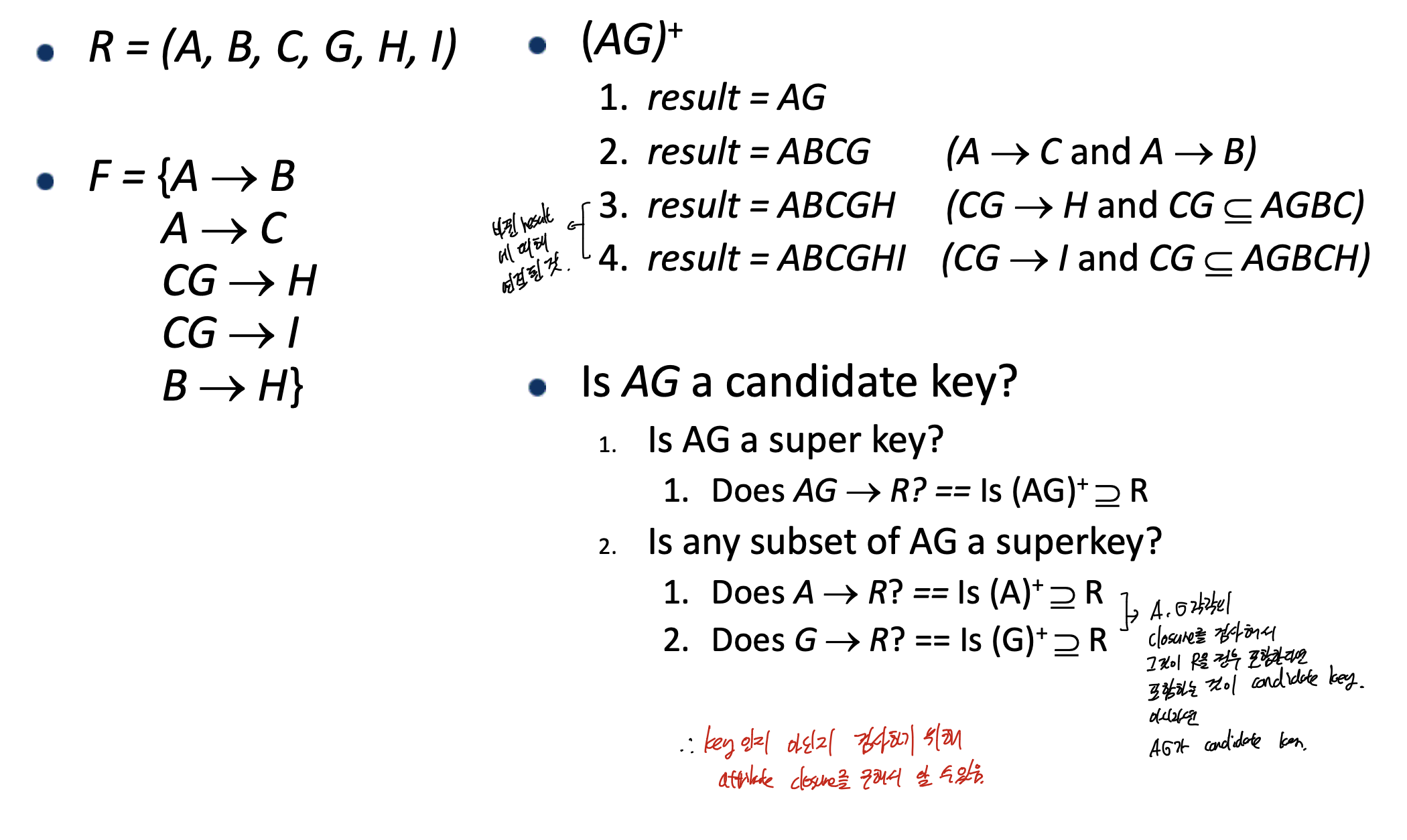
이렇게 attribute closure를 이용해서 key인지 아닌지 구할 수 있다.
AG+를 구하면, ABCGHI가 나온다.
그리고 이것이 candidate key인가. 라는 질문이 오면, 우선 AG가 super key인지 부터 구해야 한다. 여기에선 A+에 R이 다 들어가 있으니 superkey이다.
그리고 A, G가 R을 정하는지에 대해 구해야 한다.
이것은 추가적으로 A+, G+를 구해 이것이 R을 결정하는지를 확인해야 한다.

고로 key인지 아닌지 확인하기 위해 attribute closure를 구해 확인할 수 있다.

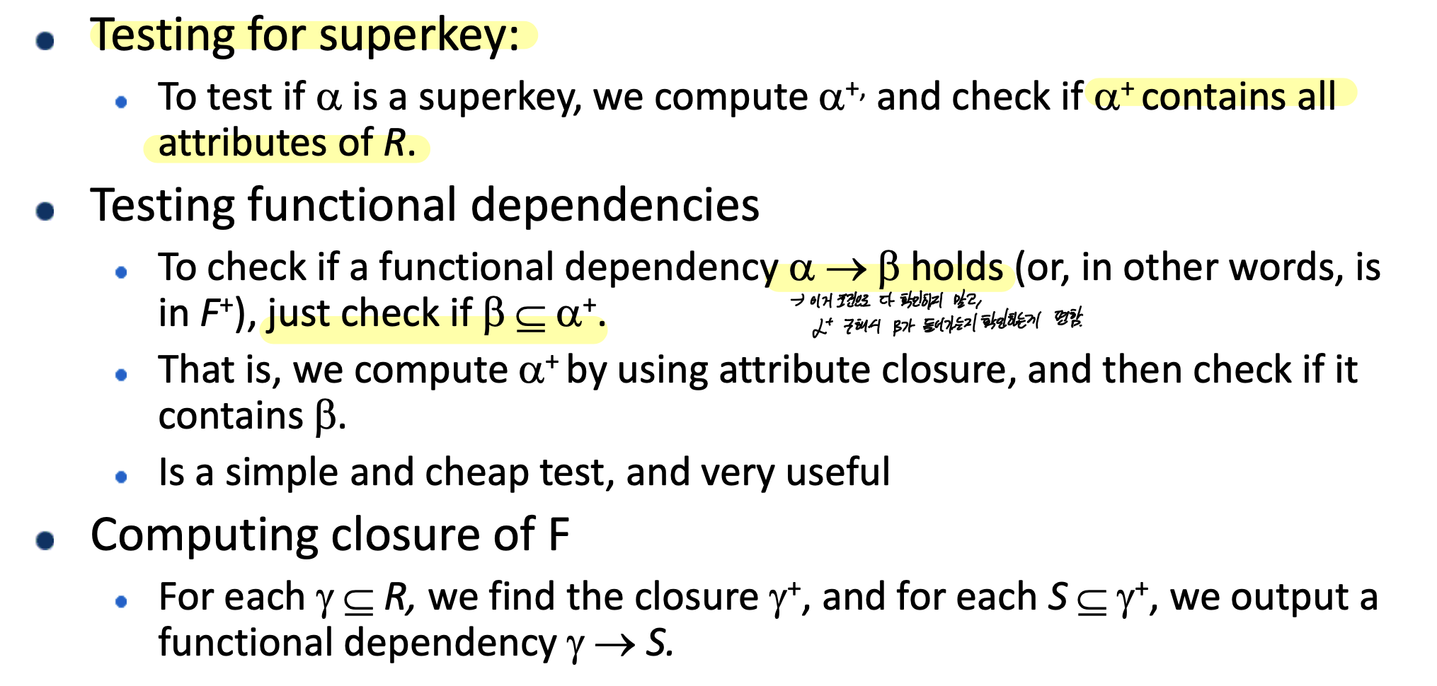
이렇게 superkey인지 확인, 그리고 functional dependencies를 확인하는데 쓸 수 있다.

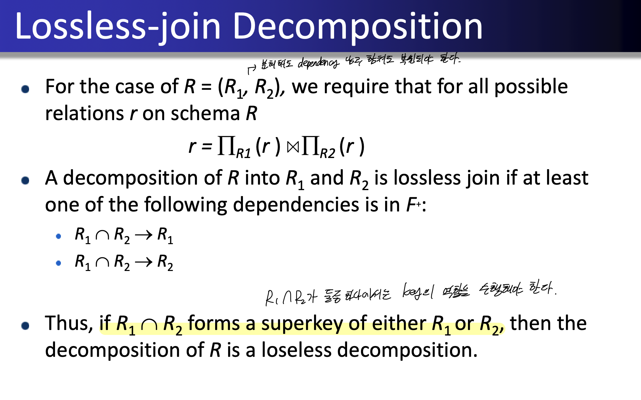
이렇게 분해했을때, R1, R2의 교집합이 둘중 하나에서는 superkey 역할을 수행해야 lossless decomposition이라 할 수 있다.

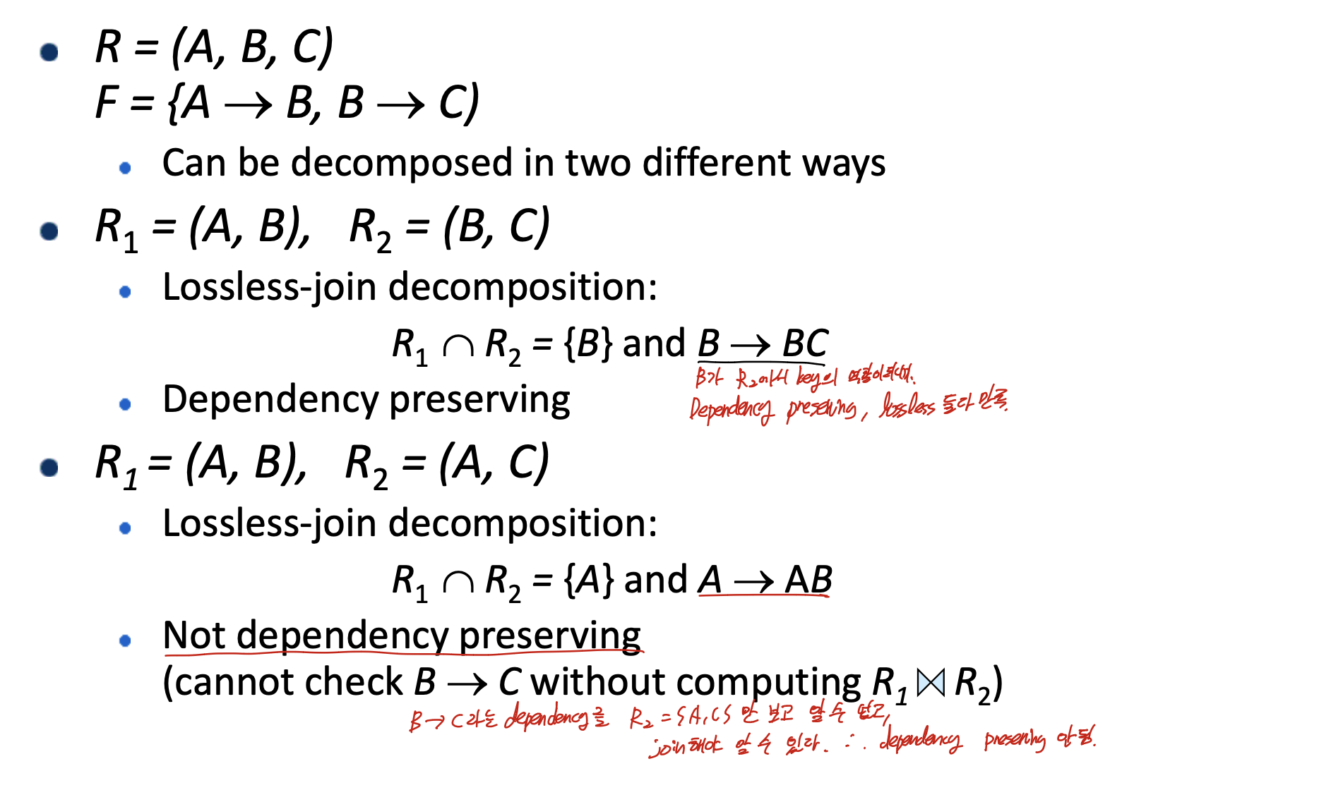
이 예시를 보고 알 수 있는데, 일단 AB, BC로 나누면 B가 R2에서 superkey 역할을 한다. 그러므로 lossless이고, Dependency를 전부 만족 한다.
하지만 두번째에서는 A -> AB이므로 lossless는 만족하지만, B ->C가 join하지 않은 상태로는 알 수없으므로 dependency preserving을 만족하지 않는다.

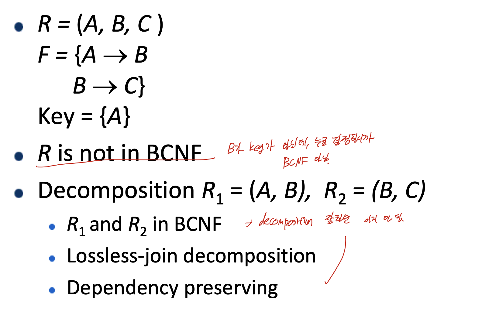
이렇게 잘 나누면 다 만족한다.
key가 아닌 것이 다른것을 결정하므로, BCNF가 아니다.!!

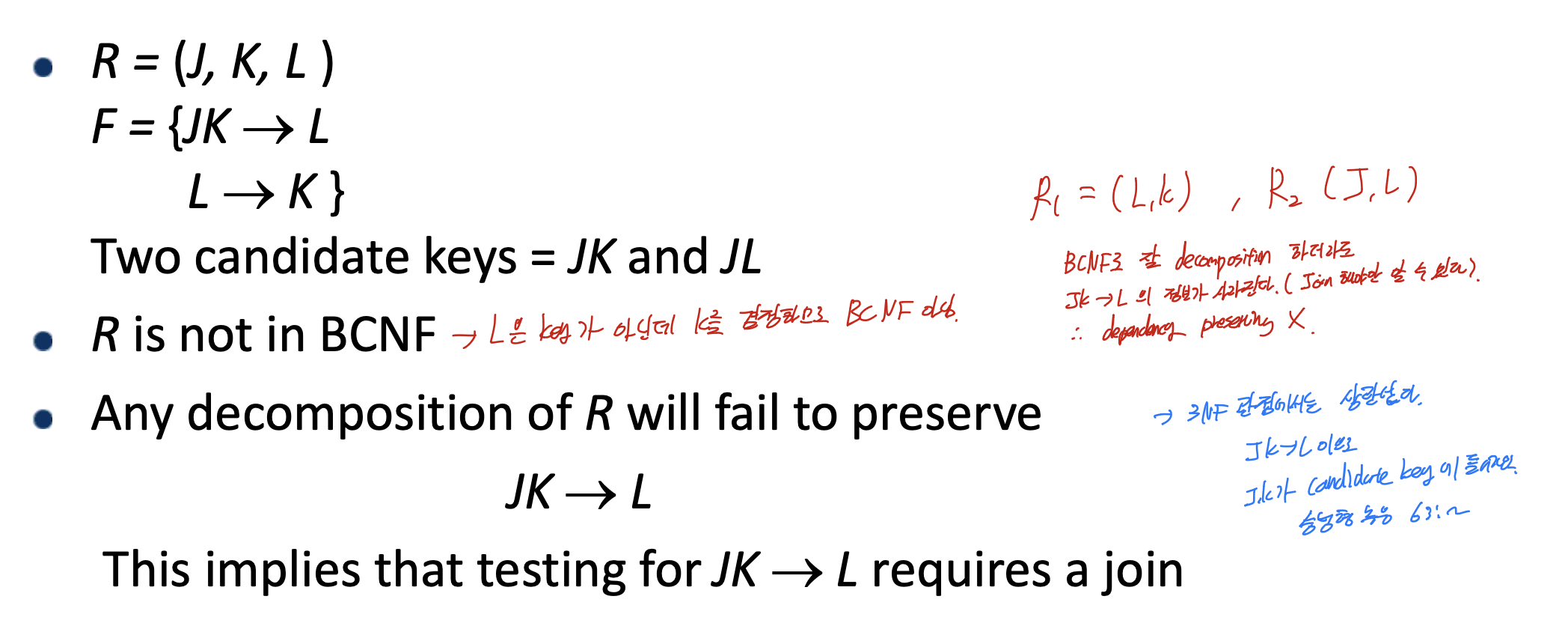
키가 아닌 L이 다른것을 결정하므로 , BCNF가 아니다.
3NF는 맞다. JK->L->K인데,

3NF에서는 lossless decomposition, dependency preserve가 항상 가능하다.
반면, BCNF에서는 Lossless는 가능한데, Dependency preserve가 안될 수 있다.

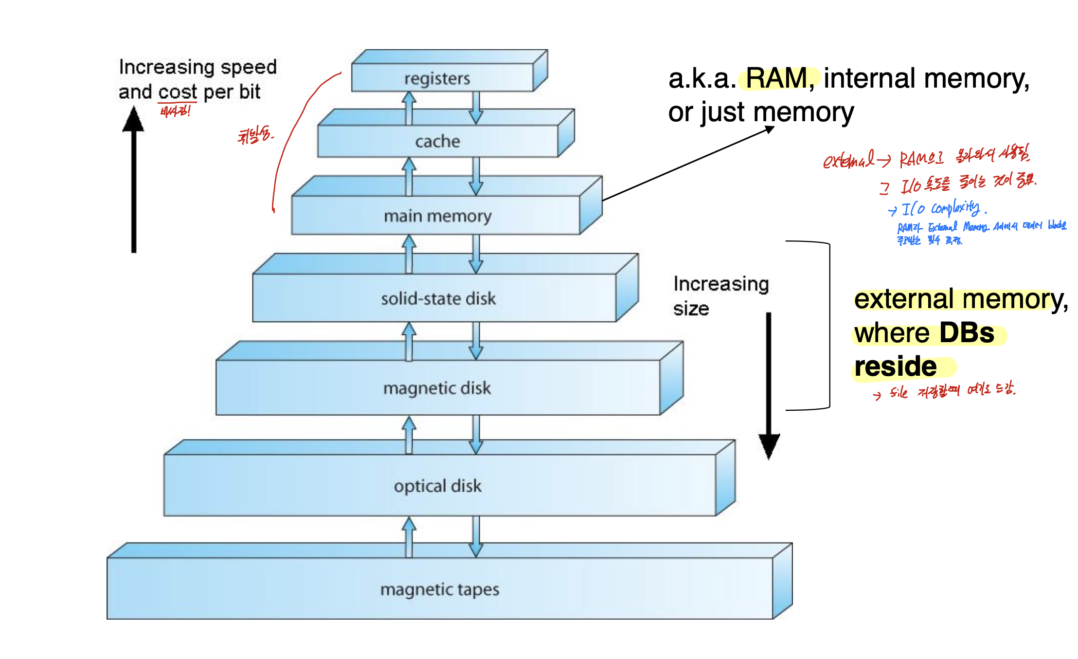
Storage and file system

file <- block <- record <- field

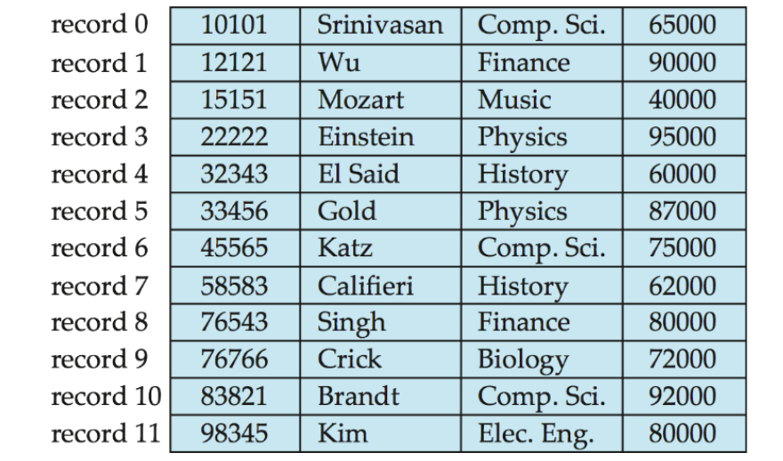
fixed length record
file의 각 레코드들이 비어있지 않고, sequential을 유지.

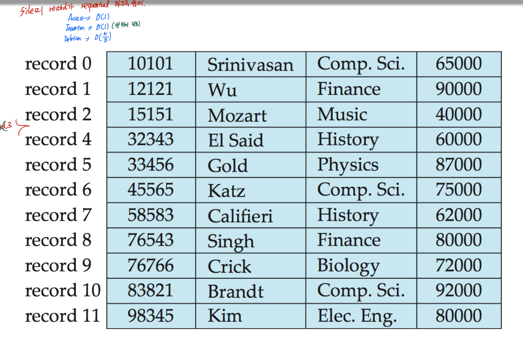
이렇게 항상 sequential 해야 하므로, 하나가 지워지면 앞으로 다 민다.
그러므로 access -> O(1), insert -> O(1)마지막에 넣으면 되니까.
delete -> O(N/B)선형시간

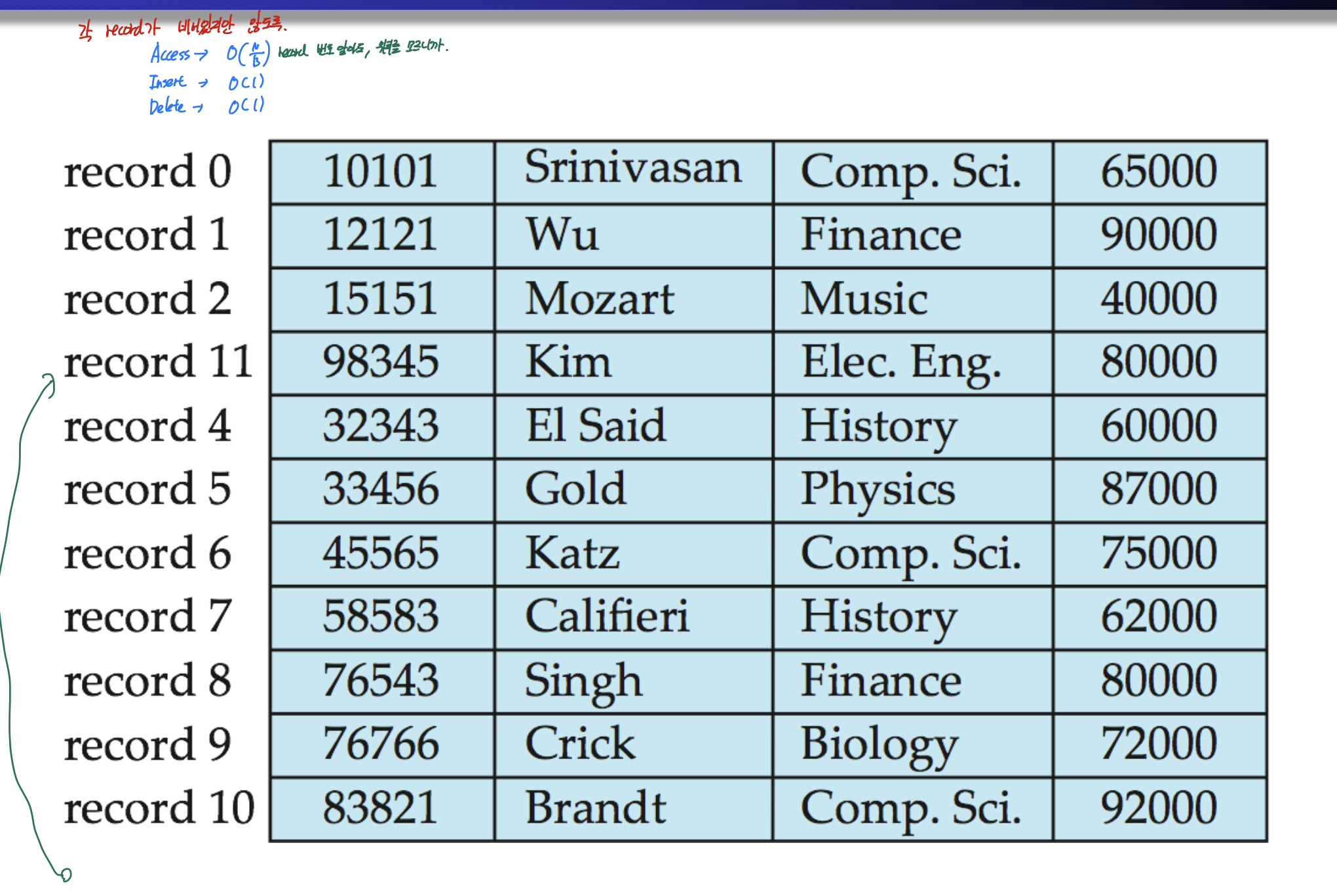
이건 fixed length record 중에, 각 레코드가 비어있지만 않도록 하는 것 이다.
접근은 각 레코드의 위치를 모르니까 O(N/B), insert는 O(1) 빈곳에 들어가니까, delete는 O(1) 그냥 빼주면 되니까

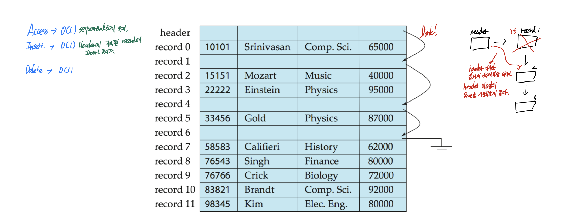
비어있는 공간을 free list로 linked list 형식으로 바꾸어 주는 것이다.
이러면 우선 header 다음을 잡아서 insert하면 O(1), delete하고 list 마지막에 넣어주면 O(1), sequential order를 만족하니까 access O(1)ㅣ이다.

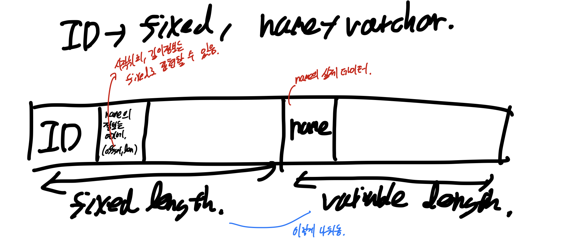
fixed length record
일단 record 하나를 나타낸 것 이다.
Fixed part에는 시작번호와, 길이정보가 들어간다. 그리고 variable part에 데이터가 들어간다.
그리고 Null bitmap으로 데이터가 null인 곳의 번호를 기록한다(?)

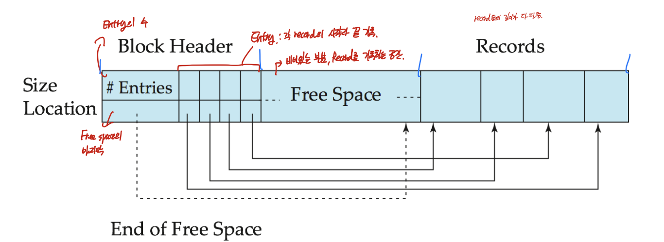
block 안에서는 이렇게 그려진다. Entry들의 수, free space의 마지막 주소, 그리고 각 record의 시작과 끝을 기록한 entry, 그리고 record가 기록된다. record는 오른쪽부터 들어오고, entry는 왼쪽부터 들어온다.

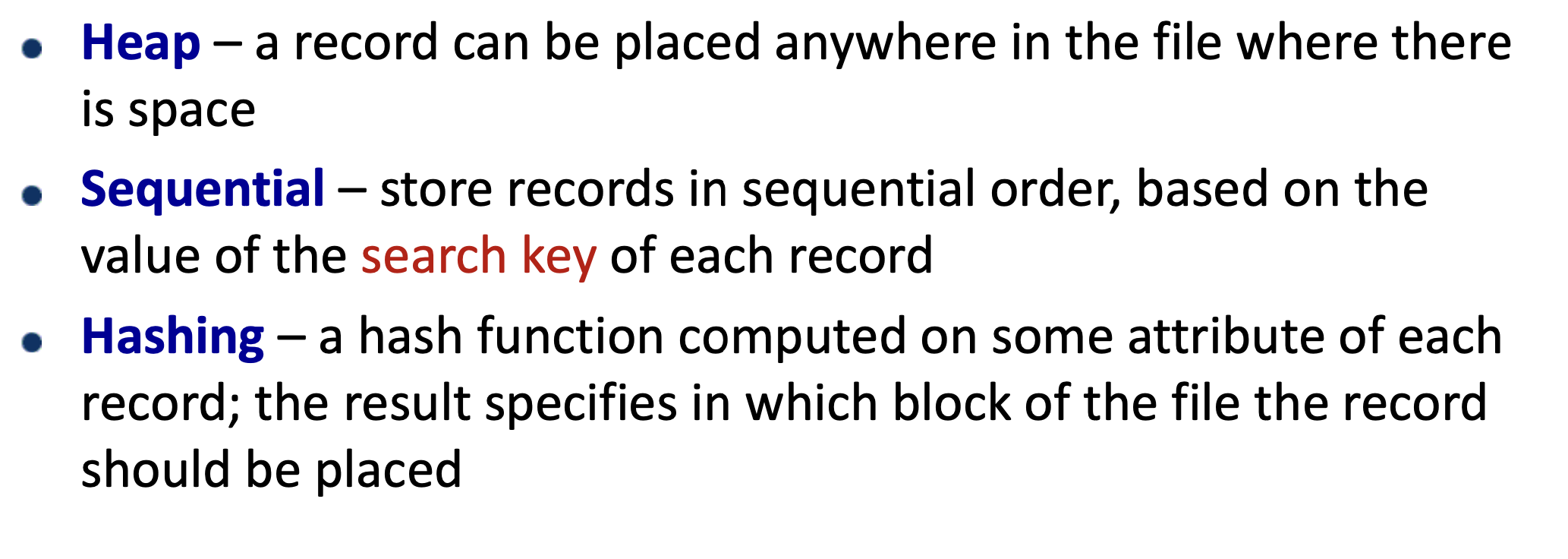
file안에 block을 배치하는 방법.

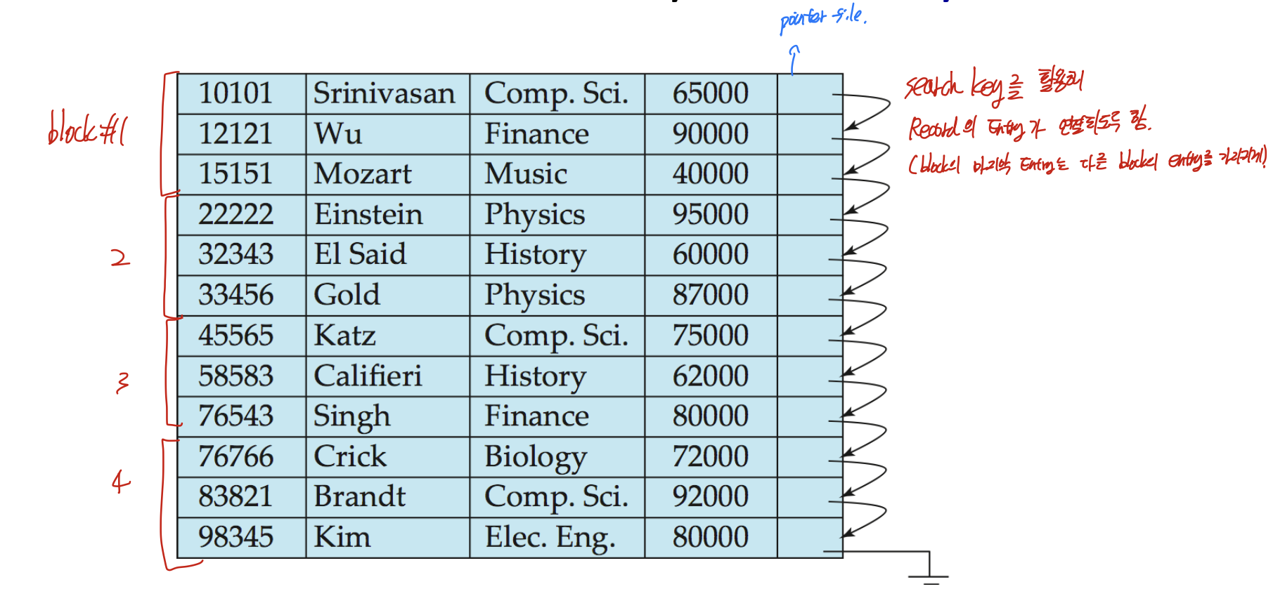
이중 Sequential file organization은 이렇게 수성된다.
search key를 활용하여 정렬을 하도록 하고, pointer file을 이용해 각 block이 연결되도록 한다.(block의 마지막 entry는 다음 block을 가리키게)

이 sequential file에서는,
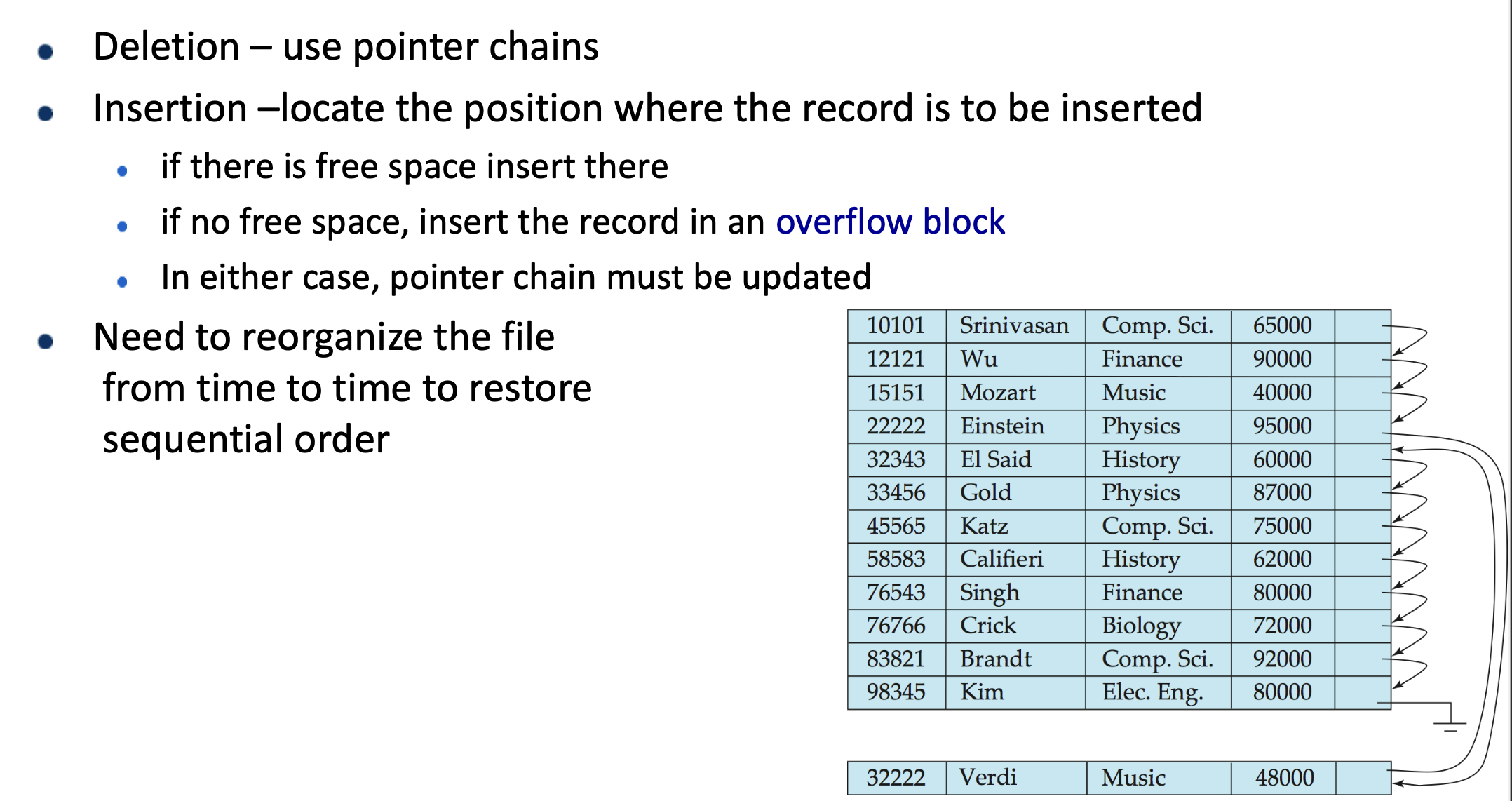
deletion은 우선 pointer chain으로 구성하면 되므로 삭제된 record가 포함된 entry 간의 포인터 정보를 바꾸면 된다. 그러므로 O(1)
insertion은 search key의 순서에 맞게 넣고, 포인터 조정을 하면 되므로 O(1)이다. free space가 있으면 바로 insertion을 수행하고, free space가 없다면 overflow block을 새로 만들어 저장한다.

access는 이미 search key의 순서로 정렬되어 있으므로, 이분탐색을 수행하여 O(logN/B)가 걸리게 된다.

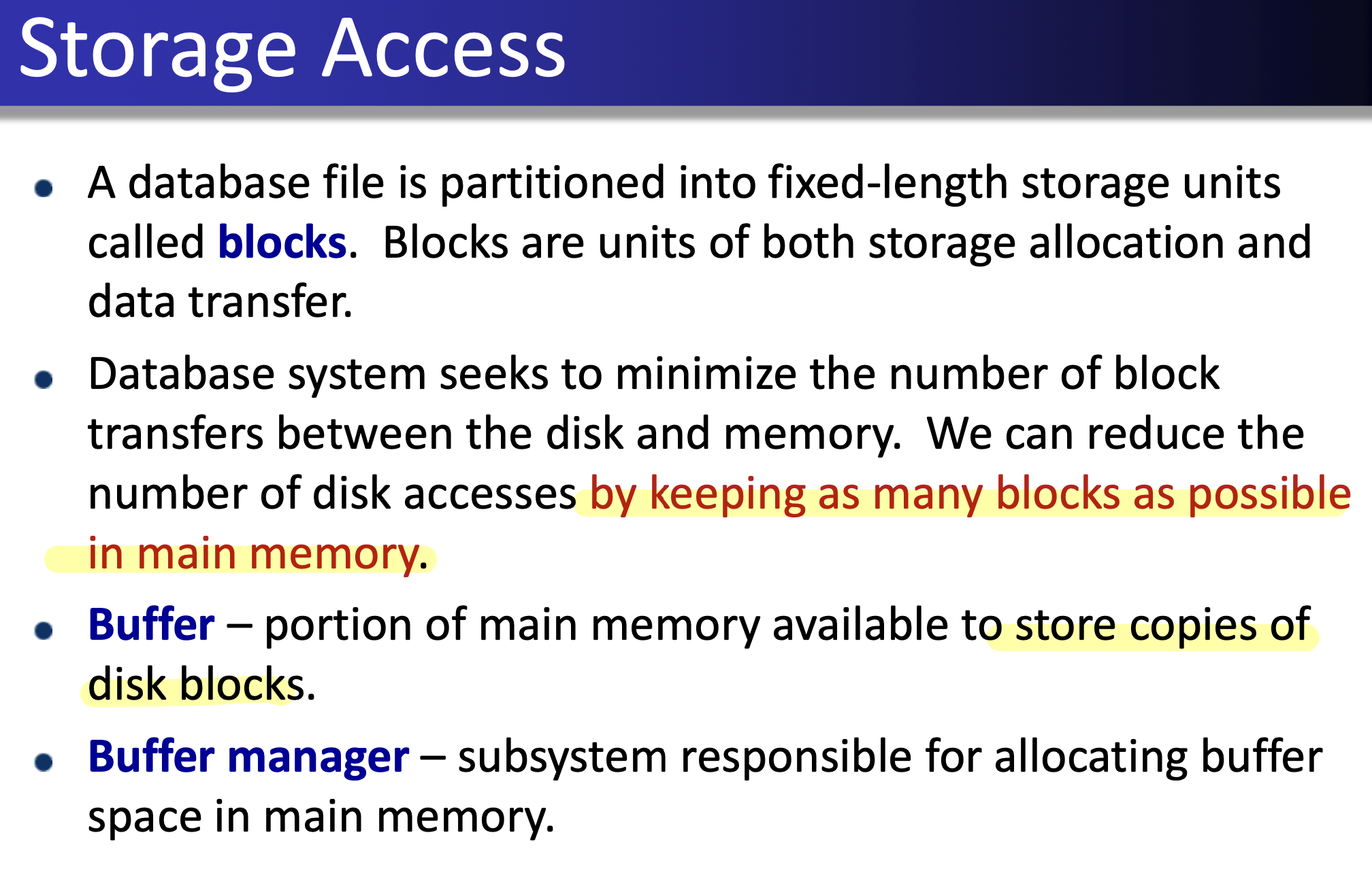
데이터를 찾는 시간을 줄이기 위해, 최대한 많은 데이터를 메모리에 올려놓는 것이 중요하다.
그걸 위해 Buffer manager를 사용한다.

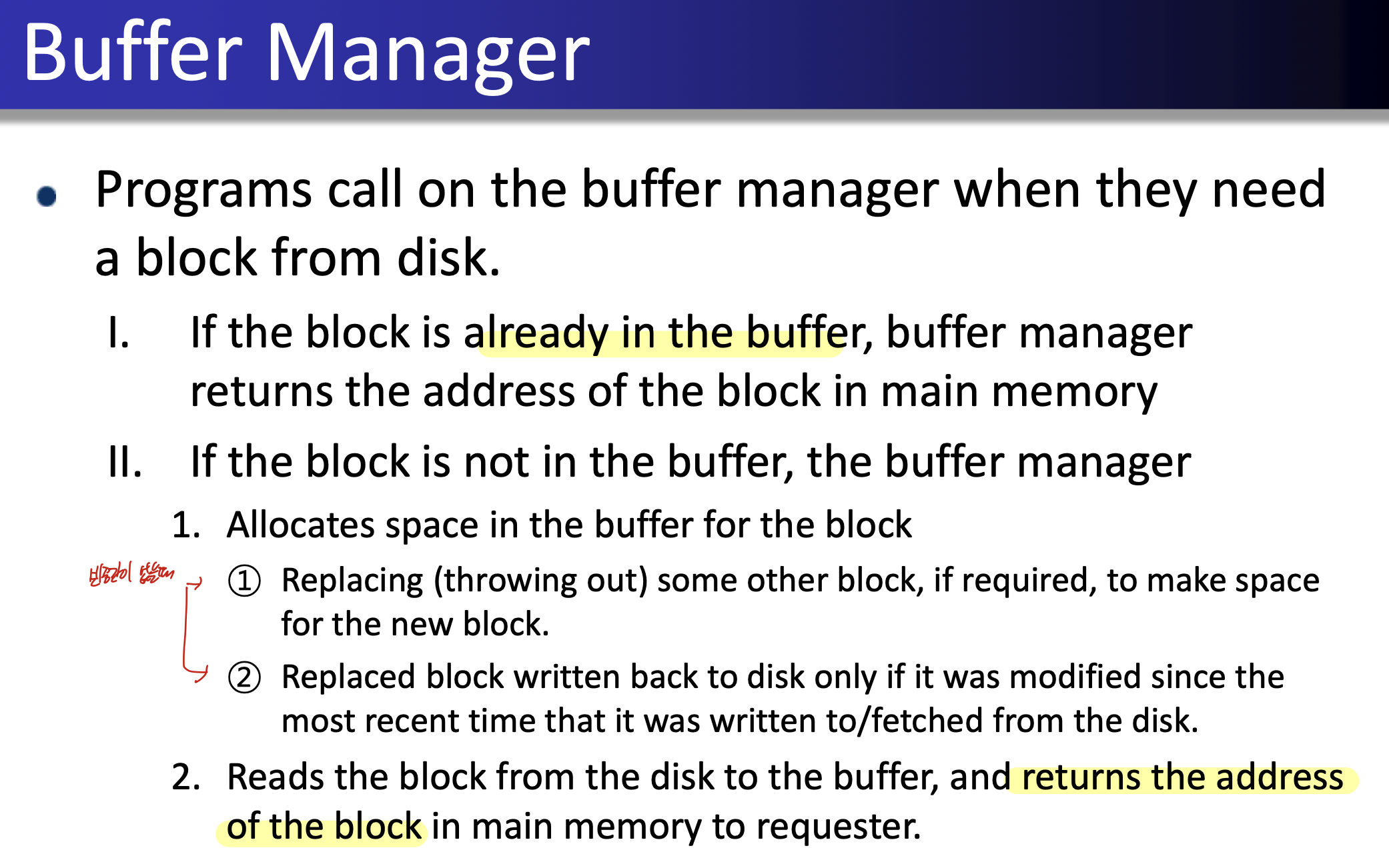
buffer manager의 동작 과정.
만약 block이 buffer에 이미 있다면, 그 블락의 주소를 리턴.
버퍼에 없다면, 공간이 필요하다면 victim을 선정해 교체하고, 공간이 있으면 insert한다. 만약 변경되었으면, 다시 disk에 옮겨준다.

LRU랑 MRU있는데, 두개가 반대임.

Indexing

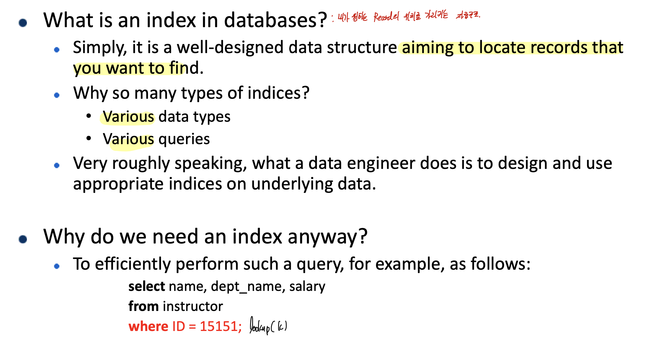
index -> 내가 원하는 record의 위치를 가리키는 자료구조.
효율성을 위해 사용.

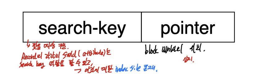
index는 searchkey와 pointer로 구성되어 있다.
searchkey는 record의 각각의 field, 즉 arrribute가 사용될 수 있고 pointer는 block 내에서의 record의 실제 위치를 나타낸다.
ordered index, hash index 두종류가 있다.

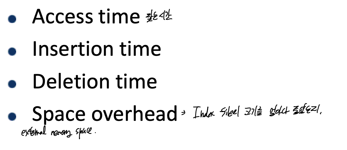
index에 대한 평가기준이다.

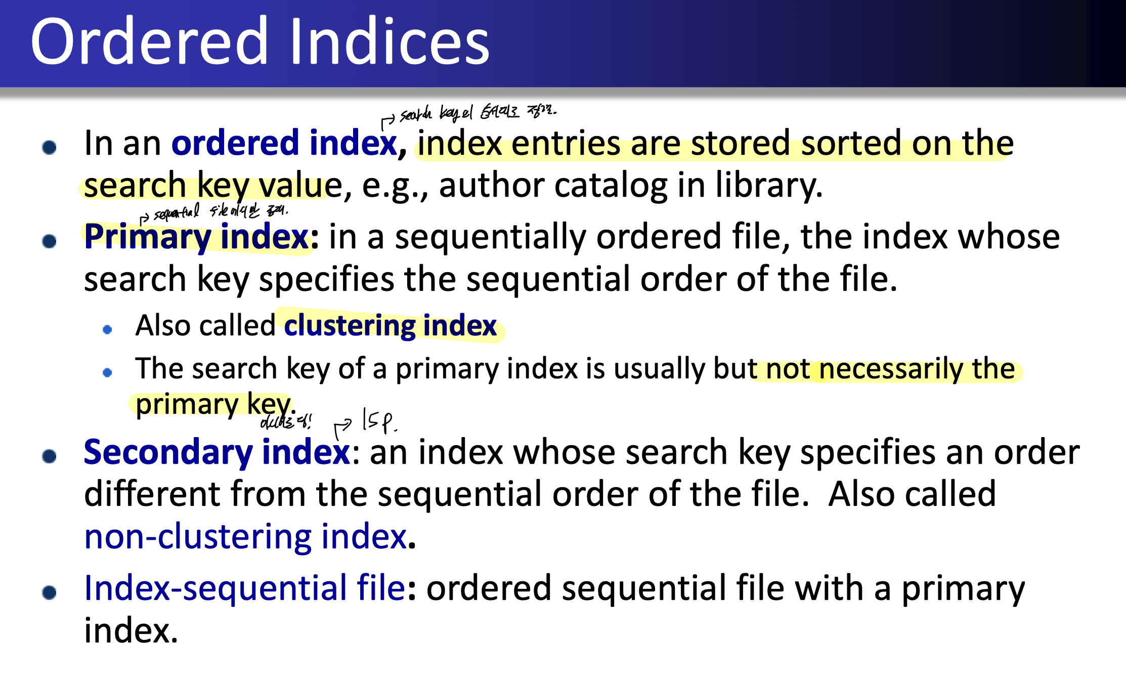
ordered index는 index entry가 search key value로 정렬되어 있는 것 이다.
primary index는 순차적으로 정렬된 파일에서, index의 search key가 파일의 sequential order를 특정하는 것 이다. (clustering index라고도 부른다.), 꼭 primary key일 필요는 없다. primary index로 정렬된 파일을 index-sequential file이라 한다.
secondary index는 그렇지 않다.

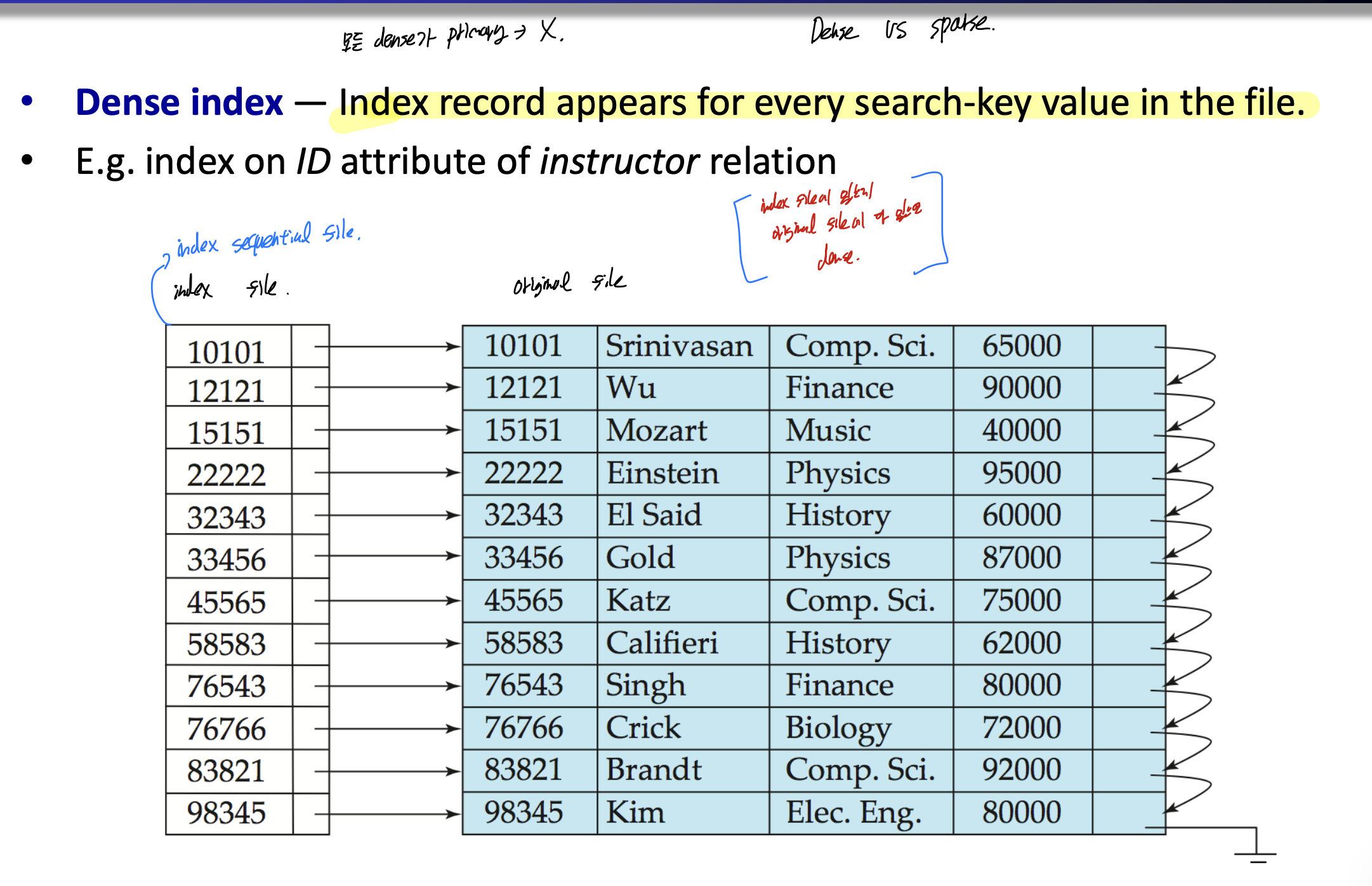
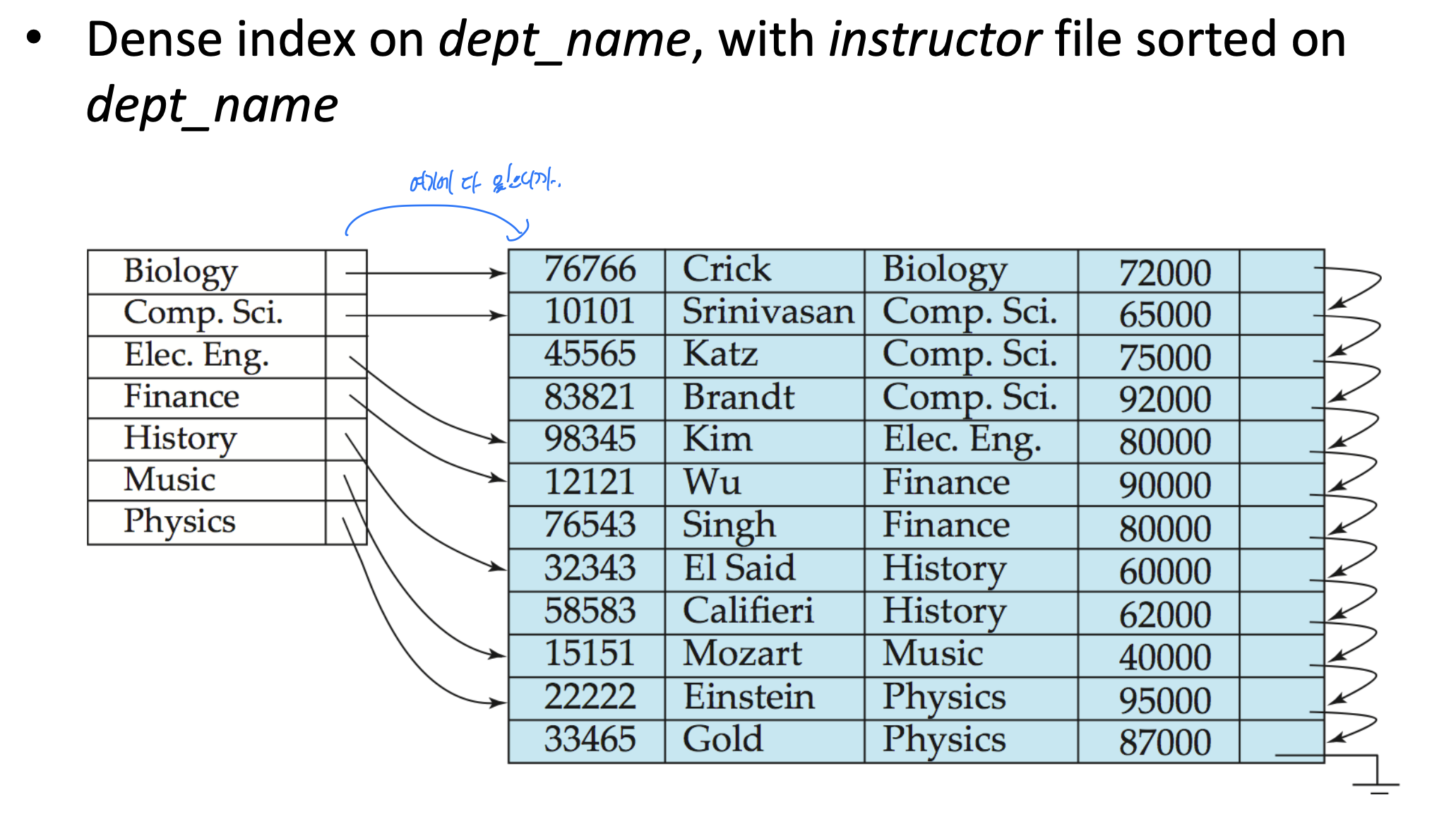
Dense index이다.
index가 file에서의 모든 search key value를 가지고 있어야 한다.
index file에 있는게 original file에도 다 있으면 dense이다.

모든 Secondary는 dense여야 한다.
모든 dense는 primary가 아니다.

이렇게 index file안에 있는 것이 original file에 다 있으므로, dense이다.

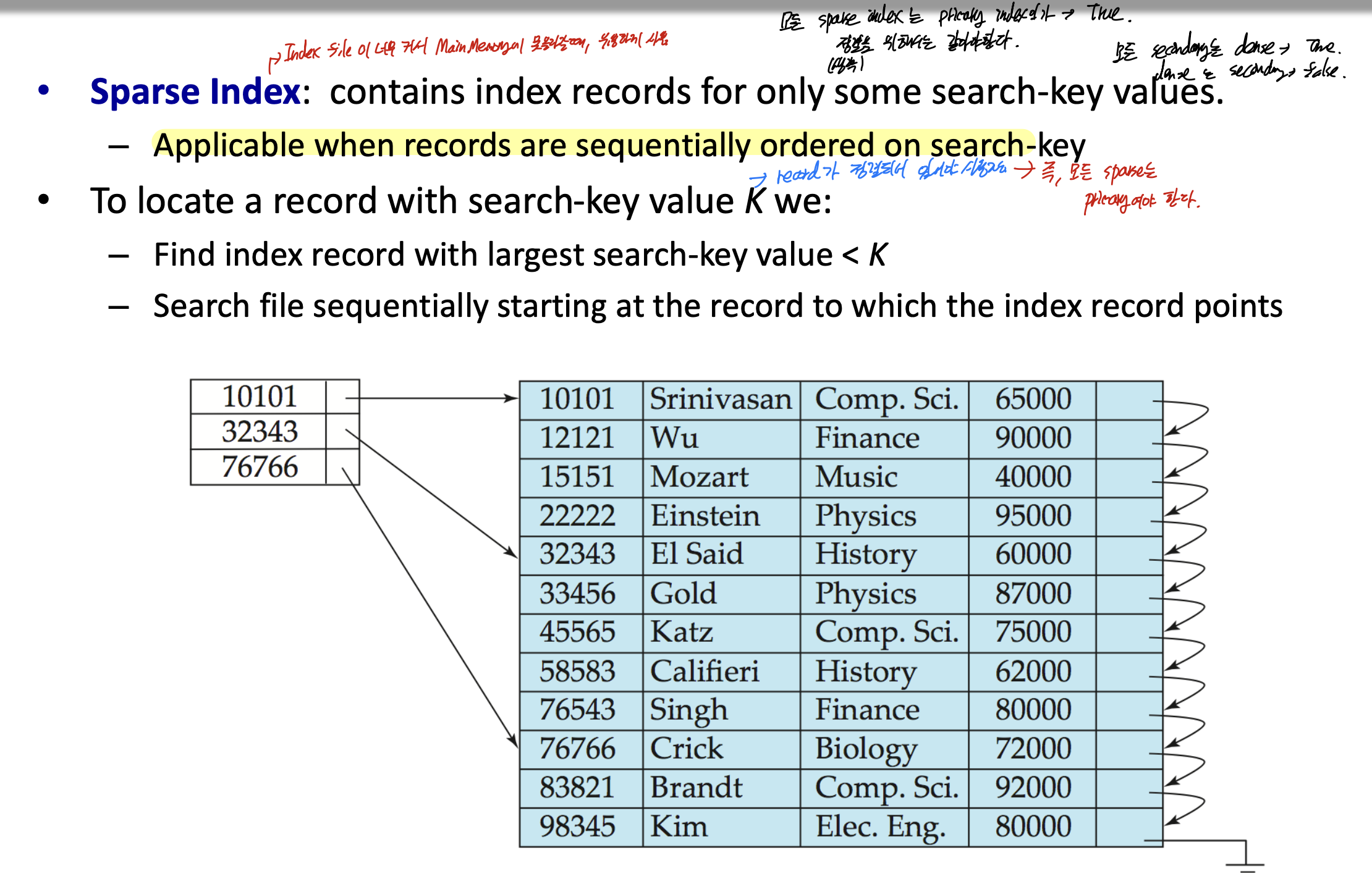
sparse index -> index file이 너무 커서 main memory에 저장하기 힘들때 유용하게 사용할 수 있다.
index file에 search key의 일부만 넣어놓는 것 이다.
항상 sequentially order를 만족해야 하기 때문에, 모든 sparse는 primary이다.

sparse는 dense에 비해 record를 놓는 시간은 오래 걸리지만, 공간적 이득을 많이 볼 수 있다.

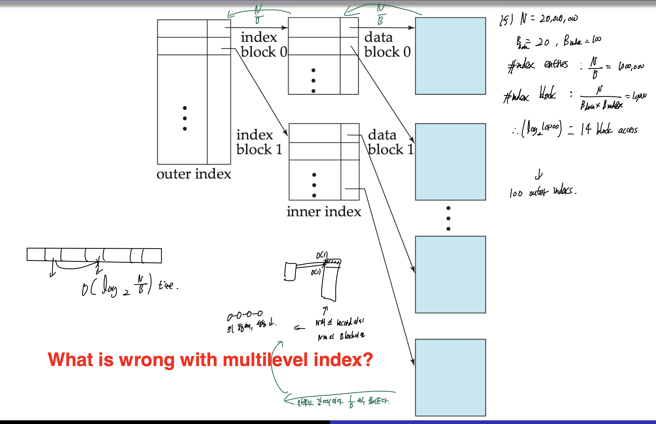
primary index가 memory에 맞지 않는다면, access하는데 많은 비용이 들 수 있다.
그러므로 위 그림처럼 multilevel index로 해준다.
inner index는 primary index file이고, outer index는 sparse index for primary index이다.
여기서 block access time은 O(logN/B)가 걸린다.
N이 20000000이라 하고, B data = 20, B index = 100이라 하자.
그러면 index entry(전체 블락의 개수)는 1000000개가 나오게 된다. 이때의 index block이 100개이므로, outer index는 100개가 되고,
그러므로 접근 시간은 log2 10000 -> 14 block access가 필요하게 된다.

블락 안에 데이터의 개수 20
-> index entry의 개수 -> N/B -> 1000000
index entry 가 하나의 블락에 100개가 들어감. -> index block -> 10000
10000개의 block을 가리키기 위해서는 index block 하나에 100이니까 100개가 들어감. -> outer index = 100
multilevel index는 N개의 record인데 N개의 block으로 나눌떄, 성능이 안좋아짐.

Index deletion

dense에서는 그 index가 가리키는 모든 Record가 삭제되었을때 그 index를 삭제.
sparse에서는 만약 search key가 index에 있다면, 다음 search key를 index로 교체한다.
만약 다음 search key도 또한 index에 있다면, 그냥 삭제.

Insertion

dense에서는 만약 그 search key가 index에 없다면, 넣어준다.
sparse에서는 순서에 맞게 record가 들어가고, index에는 다른 변화가 없다. 하지만, 그 insertion으로 인해 새로운 block이 생길 경우 새로운 블럭에 넣고, 그 search key를 index에 넣어준다.

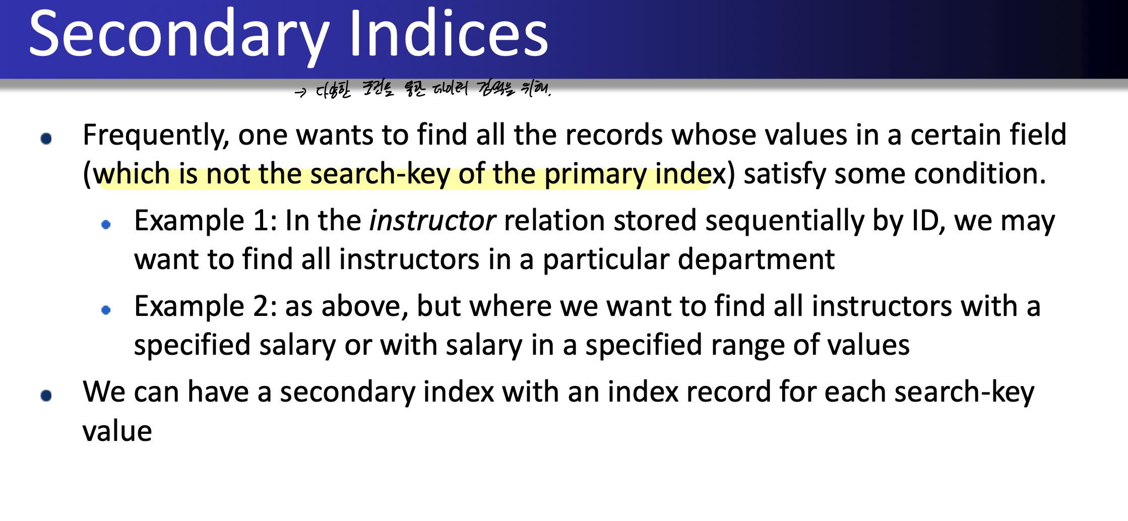
secondary index -> 다양한 조건을 통한 데이터 검색을 위해.

B+ tree

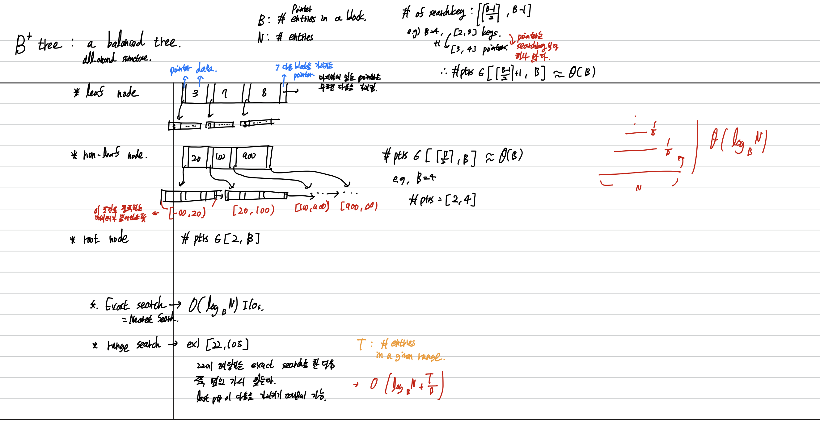
N -> record의 개수.
B -> pointer의 개수.

leaf node
포인터 -> 실제 데이터를 가리킨다. sparse일 수 도 있고, dense일 수도 있다.
마지막 포인터는 다음 leaf node를 가리킨다.
leaf node는 searchkey의 개수로 평가한다. 고로, [B-1/2, B-1]개의 search key를 가지고 있어야 한다.

예를 들어, 포 3 포8 포 10포의 leaf node가 있을때, [2, 3]이 된다.

non leaf node
각각의 포인터가 어떠한 범위를 나타내고 있다. 각각의 포인터는 밑으로 내려가는 block을 가리키고 있는 것 이다.
nonleaf에서는 포인터의 개수를 기준으로 한다. [B/2, B]의 범위의 포인터는 가지고 있어야 한다.
root node에서는 최소 2개는 있어야 한다.

leafnode의 개수 -> N/(B/2) -> theta(N/B)
Non leaf -> theta(N/B^2)
Height -> theta(logB N)

Exact search는
O(logB N)이 걸린다.

Insertion
Main file에 record 더해주고,
만약 leaf node에 공간이 있으면, 넣고
Overflow가 난다면 split the node
split할때는 일단 위에서부터 순서대로 들어간다.
만약 해당하는 공간의 leaf node가 가득 차있다면 , split 해준다.
N/2개는 원래에 두고, 나머지는 새로운 노드를 만들어 준다.
그리고 그 새로운 노드에 대한 nonleaf node를 추가해주는 것 이다.
만약 위에도 overflow가 난다면, 위에도 split해준다.
예시 해보기; 존나어려운데 아 ;
다섯개이면 앞에 세개 그냥 있고, 뒤에 두개 간다고 한다.

Query

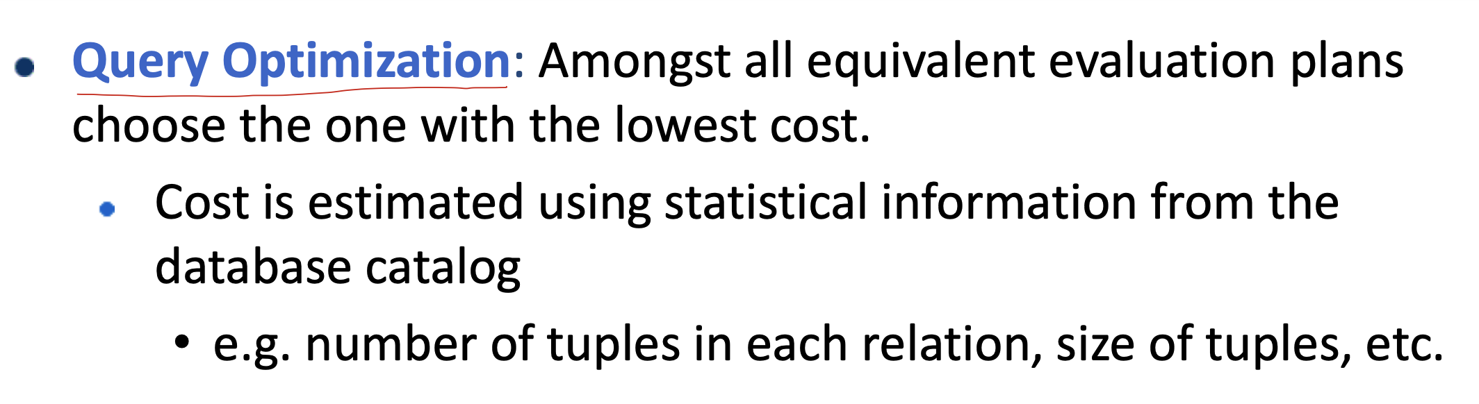
query를 최적화하는 것. 이것에 관한 알고리즘들

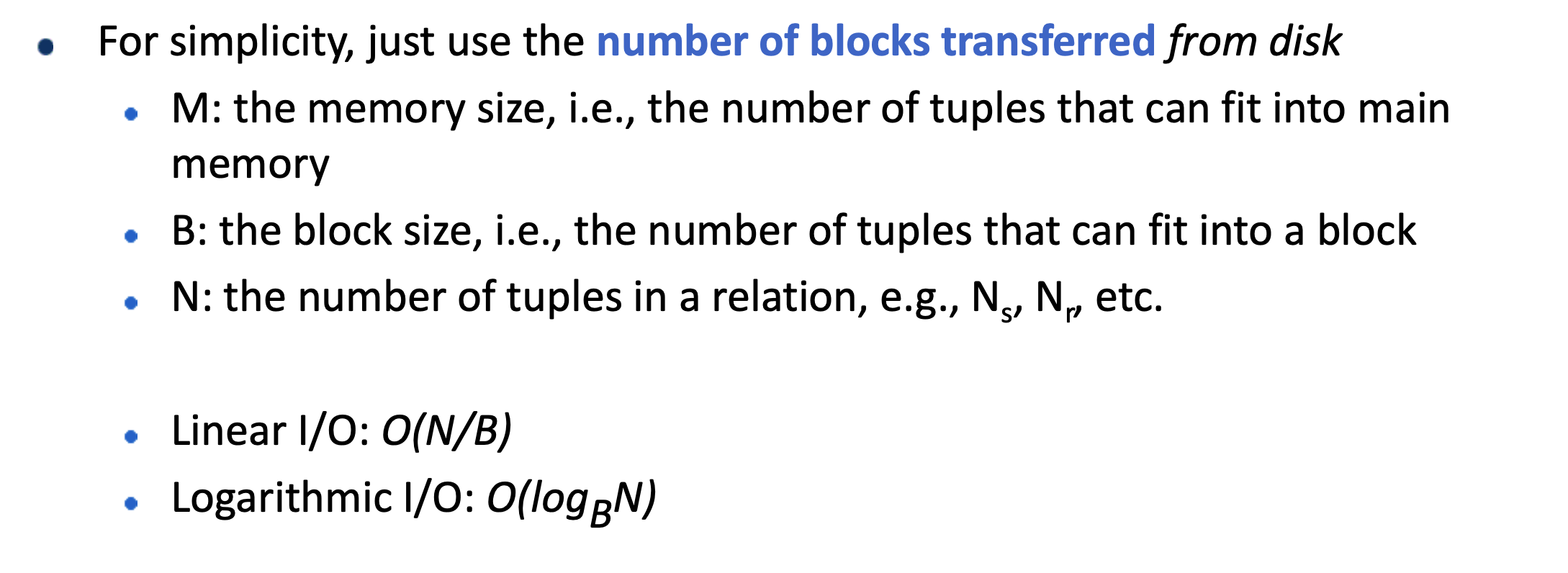
M -> memory size
B -> block size
N -> number of tuples in a relation

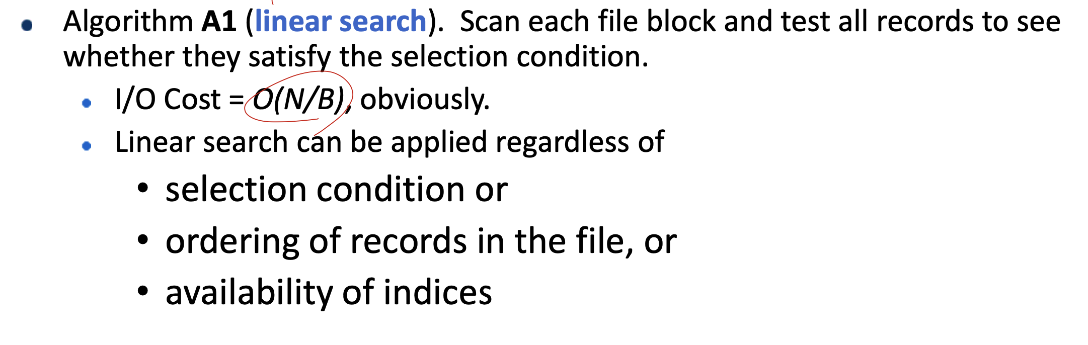
그냥 처음부터 쭉 sequential scan 하는 것 이다.
그러므로 선형시간인 O(N/B)가 걸린다.
키와 같은 경우도 sequential scan에서는 다르지 않다. 어처피 위에서부터 쭉 봐줘야된다. 그러므로 선형시간.

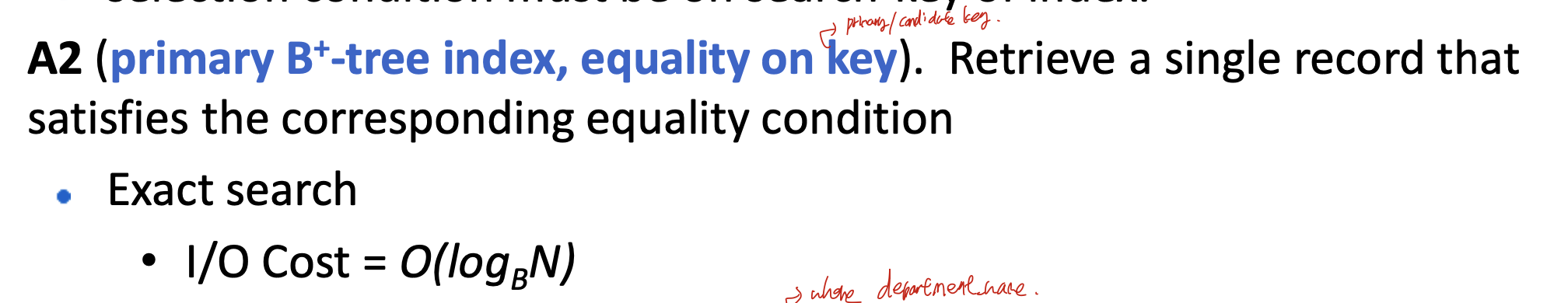
primary index가 b+ tree로 존재하며 , searchkey를 index로 사용하는 경우이다.
이 경우에서는, searchkey가 candidate key나, 다른 key인 조건을 만족하는 경우이다.
그러므로 B+ tree에서는 exact search (tree의 height)를 생각하면 된다.
그러므로 logB N 이 걸린다.

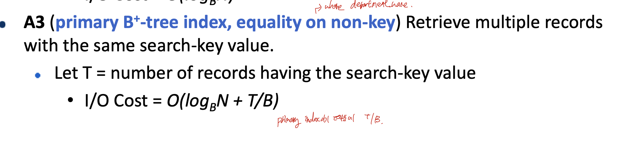
primary index가 b+ tree로 존재하지만, search-key가 candidate key 조건을 만족하지 않는 경우이다. 이 경우에는 중복된 searchkey값이 있을 수 있기 때문에, 해당하는 블록을 찾은 후 linear scan을 해야한다.
그러므로 logB N + T/B이다.
T는 쿼리를 수행해서 나왔을때 나오는 record의 수 이다.

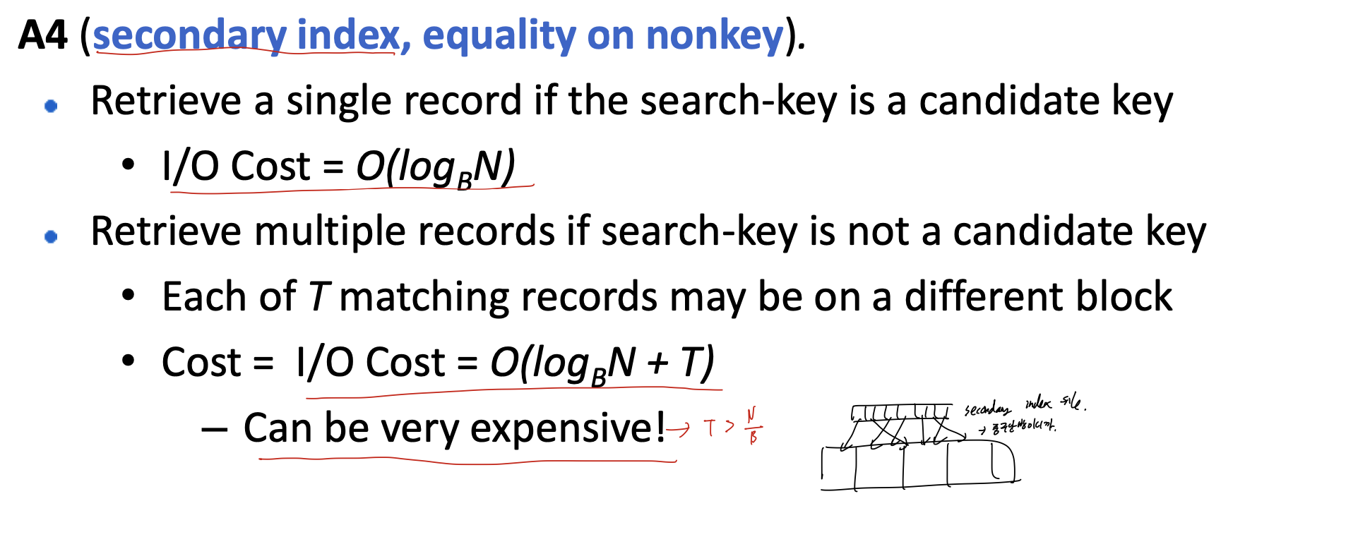
우선 A4에서 secondary index이면서 equality on key인 경우를 생각하면
search key가 key의 조건을 만족하면, A2랑 같다(order되어있기 때문).
그러므로 logB N이라고 한다.

그렇다면 searchkey가 key가 아니라면, searchkey값에 의해 정렬되어있지 않다.
그리고 secondary index이기 때문에 query 로 수행된 모든 record를 찾는 경우가 최악이다.
그러므로 logB N + T이다.
여기서 T가 N/B보다 커질 수 있어서, 비용이 많이 들 수 도 있다.

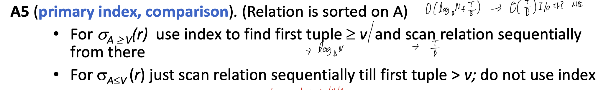
primary index에서 comparison을 수행하는 경우이다. 이 경우는 어떤 값에 의해 비교한 결과를 찾는 것이기 때문에 logB N + T/B이다.
하지만 a < 80000과 같이 이미 값이 나와있는 경우는, 그냥 linear search로 해주면 된다. 그래서 T/B로 사용할 수도 있다.

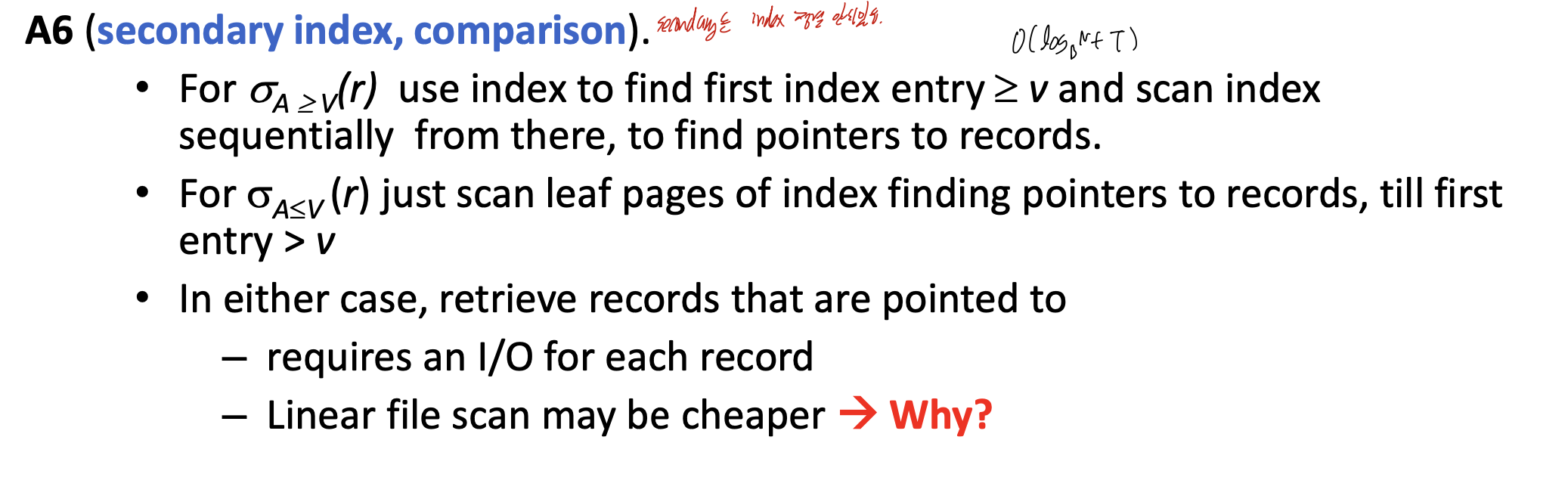
얘도 비슷하게 그래서 logB N + T이다.

External merge sort

record의 수 N이 memorysize M보다 크면, 어떻게 정렬해서 넣을 것인가?
-> external merge sort

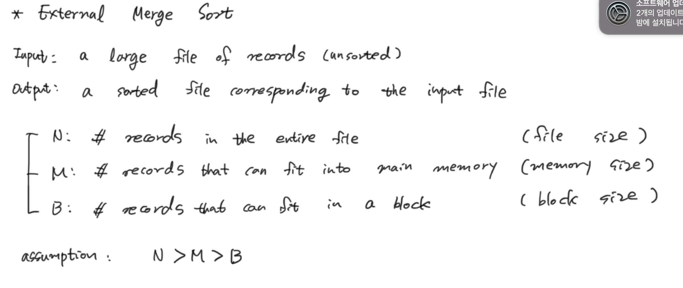
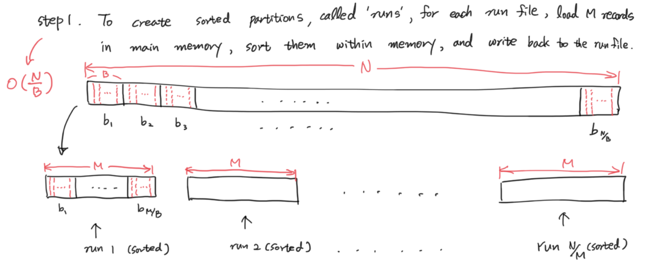
우선, M < N이므로 M size의 block들을 메모리로 가져가서 정렬하고, 다시 runfile에 돌려놓는다. 하나의 run은 M의 크기이며, M/B개의 블락을 가지고 있다. 그러므로 총 걸리는 시간은 O(N/B)가 된다. 그리고 N/M개의 initial sorted run을 가지게 된다.

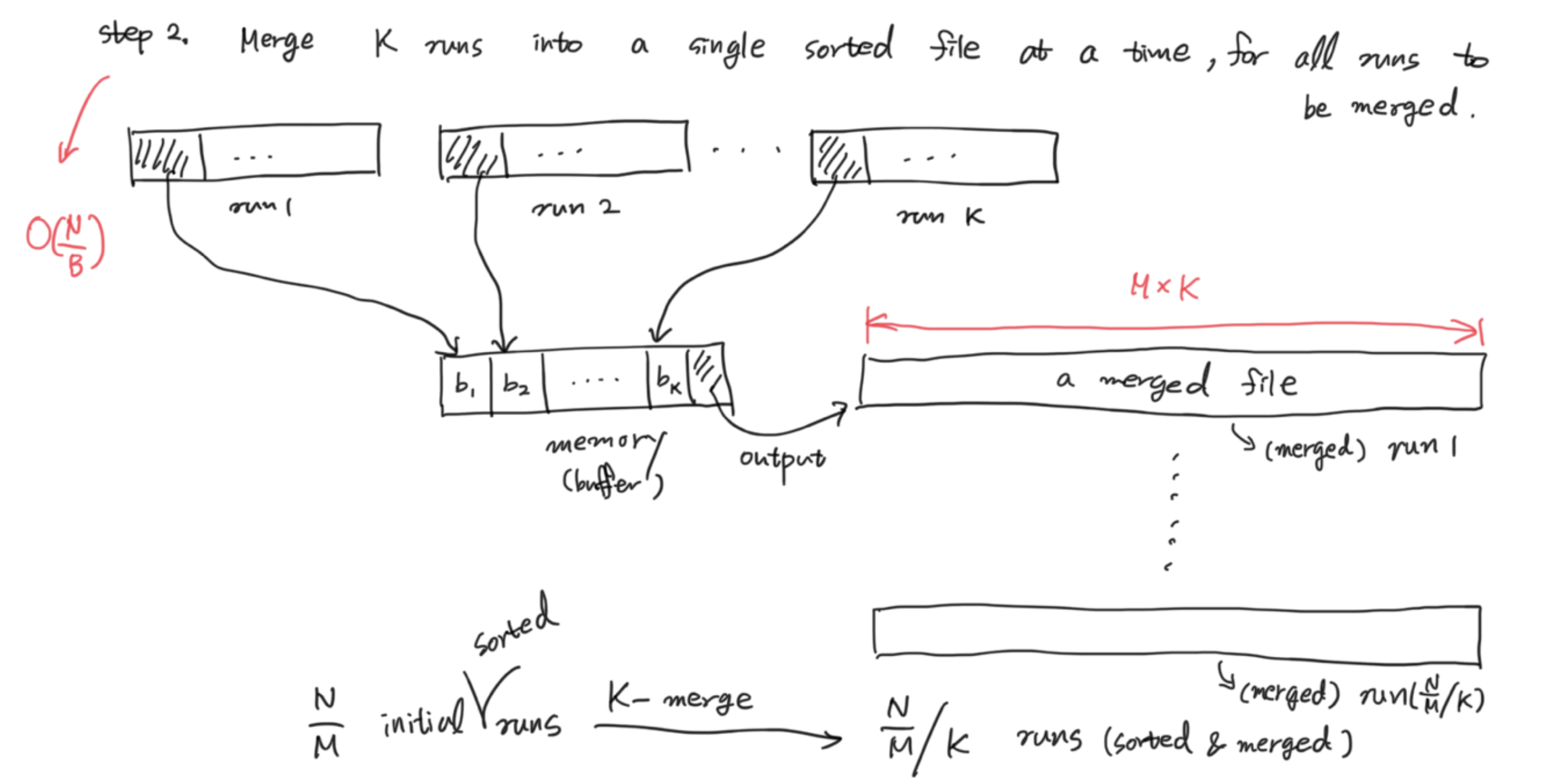
그리고 K개의 run들을 첫번쨰 block의 첫번째 record를 비교하면서 buffer에 넣어준다. 그러면 M*K개의 merged file이 생기개 되고, 이 merged file은 N/(M*K)개 이다.(O(N/B) buffer의 마지막은 항상 merged에서는 output buffer가 되어야 한다.
N/M개의 initial sorted runs가 생기고, K-merge를 통해 N/(M*K)개의 sorted, merged run이 생긴다. 이 과정을 순차적으로 해주는 것 이다.

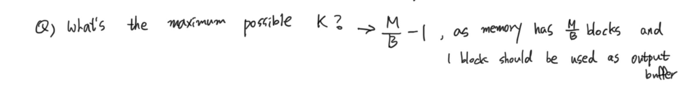
K의 최대개수는 M/B -1개 이다. M/B개의 block을 가지고 있지만, 한개는 무조건 output buffer로 사용되기 때문이다.

각 과정은 O(N/B)의 시간이 걸리고
이러한 과정이 logM/B N/M이 걸린다. 왜냐하면 N/M개에 대해서 M/B개의 블락으로 나누어 지기 때문이다.
그러므로 총 시간은 N/B * log M/B N/B이다.

dlwogns

난 커서 개발자가 될래요

DataBase (3-1)

3-1

Relational Database

bad design

Relations are not ordered

Keys

super key

candidate key

primary key

foreign key

foreign key constraint

SQL

Create

Integrity Constraints

Alter

Select

Join

as

String operation

Ordering the Display of Tuples

Where Clause Predicates

between

Tuple comparison

Set Operation

Find courses that ran in Fall 2009 or in spring 2010

Find courses that ran in Fall 2009 and in Spring 2010

Find courses that ran in 2009 but not in Spring 2010

Null Values

Aggregate Functions

group by

having

Null Values and Aggregate

Nested Subqueries

Set Comparison

some

all

exists

Not exists

unique

Derived Relations

lateral

with

Modification of the Database

Deletion

Insert

Intermediate SQL

Join

Outer Join

left outer Join

Right Outer Join

Full Outer Join

join example

View

Views Defined Using Other Views

Update of a View

Some Updates cannot be Translated Uniquely

Constraints on a Single Relation

unique

check

reference integrity

Relational DB Design

Storage and file system

Indexing

Index deletion

Insertion

B+ tree

Query

External merge sort

0개의 댓글