[Algorithm] Priority Queue를 이용한 Dijstra's Algorithm

Dijstra Alogrithm

다익스트라 알고리즘은 Dynamic programing를 이용한 최단 거리 탐색 알고리즘으로
하나의 정점에서 모든 정점으로 가는 최단 경로를 알려준다.

Priority Queue, Dijstra Alogrithm

Priority Queue를 이용한 Dijstra Alogrithm은 DP와 Greedy를 이용한 거리탐색 알고리즘이다.

다음의 그림의 그래프를 살펴보자

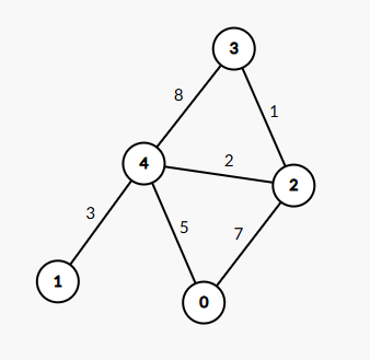
정점 0에서 시작해 모든 정점의 최단 거리를 구해보자.

사전준비
1. 0에서 다른 정점으로 가는 최단 거리 배열을 만든다.
2. 방문해야할 노드의 정보를 담은 우선순위 큐를 만든다. 우선순위 큐는 최소 힙(Min-Heap)을 사용하여 현재 최단 거리를 가진 노드를 빠르게 가져올 수 있도록 한다.

Node	0	1	2	3	4
dis	0	INF	INF	INF	INF

Priority Queue: (노드: 0,거리: 0)

Step1
우선순위 큐에서 노드 0을 꺼내온다.

0에서 인접한 노드는 4,2이고 최단거리를 구하면 다음과 같다.
최단거리는 (dis[현재노드] + 현재노드와 인접노드의 가중치)와 dis[인접노드]의 최솟값으로 구한다.

Node	0	1	2	3	4
dis	0	INF	7	INF	5

만약에 인접한 노드의 최단거리가 갱신이 되면, 우선순위 큐에 넣는다. 여기서 dis[4]와 dis[2]가 모두 갱신되었으므로 2와 4를 우선순위 큐에 넣는다.

Priority Queue: 4, 2

Step2
우선순위 큐에서 최단거리가 가장 작은 노드4를 꺼낸다.

4와 인접한 노드는 0,1,3,2이고 최단거리를 구하면 다음과 같다.

Node	0	1	2	3	4
dis	0	8	7	13	5

만약에 인접한 노드의 최단거리가 갱신이 되면, 우선순위 큐에 넣는다. 여기서 dis[1]와 dis[3]이 갱신되었으므로 1와 3를 우선순위 큐에 넣는다.

Priority Queue: 2, 1, 3

Step3
우선순위 큐에서 최단거리가 가장 작은 노드2를 꺼낸다.

인접한 노드는 0,3,4이고 최단거리를 구하면 다음과같다.

Node	0	1	2	3	4
dis	0	8	7	8	5

만약에 인접한 노드의 최단거리가 갱신이 되면, 우선순위 큐에 넣는다. 여기서 dis[1]와 dis[3]이 갱신되었으므로 3를 우선순위 큐에 넣는다.

Priority Queue: 1, 3, 3

Step4
우선순위 큐에서 최단거리가 가장 작은 노드 1를 꺼낸다.

인접한 노드는 3이고 최단거리를 구하면 다음과 같다.

Node	0	1	2	3	4
dis	0	8	7	8	5

만약에 인접한 노드의 최단거리가 갱신이 되면, 우선순위 큐에 넣는다. 여기서 갱신된 값이 없으므로 큐에 아무것도 넣지 않는다.

Priority Queue: 3, 3

Step5
큐의 남은 부분도 처리해주면 다음과 같이 나올 것이다.

Node	0	1	2	3	4
dis	0	8	7	8	5

DP와 Greedy인 이유

1. Dynamic Programming(DP)의 이유
   DP의 핵심은 작은 문제를 풀고 그 결과를 재사용해서 큰 문제를 푸는 것이다.
   dis[node] 배열은 각 노드까지의 최단 거리를 저장해서 이후 계산에서 재사용함.

2. Greedy(그리디)의 이유
   그리디의 핵심은 매 단계에서 최선의 선택을 하면서 전체 문제를 푸는 것이다. 다익스트라 알고리즘에서는 현재 방문하지 않은 노드들 중에서 "최단 거리"를 가진 노드를 매번 선택해서 처리한다. 이는 우선순위 큐를 사용해 가장 짧은 거리의 노드를 선택하여 처리한다.

시간복잡도

1. 노드 처리 시간
   • 노드의 개수를 V(Vertices, 정점)라고 할 때:
   • 각 노드는 한 번만 큐에서 꺼내지므로, 큐에서 꺼내는 연산은 최대 V번 발생.
   • 우선순위 큐에서의 "꺼내기" 연산의 시간 복잡도는 O(log V).
2. 간선 처리 시간
   • 간선의 개수를 E(Edges, 간선)라고 할 때:
   • 각 간선은 최대 한 번 "탐색"되고, 그 과정에서 큐에 삽입될 수 있다.
   • 큐에 값을 삽입하는 연산의 시간 복잡도는 O(log V).
   • 따라서, 간선 처리는 최대 O(E log V) 시간이 걸린다.

총 시간 복잡도
노드 처리: O(V log V)
간선 처리: O(E log V)
합계: O((V + E) log V)

코드로 구현해보자

import java.util.*;
import java.io.*;

class Node {
    int v; // 노드 번호
    int cost; // 해당 노드까지의 비용

    public Node(int v, int cost) {
        this.v = v;
        this.cost = cost;
    }
}

public class Main {
    static final int INF = 100000000;

    public static void main(String[] args) throws IOException {
        int n = 5; // 노드 개수
        ArrayList<Node>[] graph = (ArrayList<Node>[]) new ArrayList[n];
        for (int i = 0; i < n; i++) {
            graph[i] = new ArrayList<>();
        }

        // 그래프 정의
        graph[0].add(new Node(4, 5));
        graph[0].add(new Node(2, 7));
        graph[4].add(new Node(1, 3));
        graph[4].add(new Node(3, 8));
        graph[4].add(new Node(2, 2));
        graph[2].add(new Node(3, 1));
        graph[3].add(new Node(1, 7));

        int start = 0; // 시작 노드

        // 다익스트라 실행
        int[] distances = Dijkstra(graph, n, start);

        // 결과 출력
        for (int i = 0; i < n; i++) {
            System.out.println("Node " + i + ": " + (distances[i] == INF ? "INF" : distances[i]));
        }
    }

    public static int[] Dijkstra(ArrayList<Node>[] graph, int n, int start) {
        int[] distances = new int[n];
        Arrays.fill(distances, INF);
        distances[start] = 0;

        PriorityQueue<Node> pq = new PriorityQueue<>(new Comparator<Node>() {
            @Override
            public int compare(Node o1, Node o2) {
                return o1.cost - o2.cost;
            }
        });

        pq.add(new Node(start, 0)); // 시작 노드 삽입

        while (!pq.isEmpty()) {
            Node cur = pq.poll();
            int curNode = cur.v;
            int curCost = cur.cost;

            if (curCost > distances[curNode]) continue; //큐에 중복된 노드처리

			//인접노드 탐색
            for (Node next : graph[curNode]) {
                int newDistance = distances[curNode] + next.cost;
                
                //최단거리 탐색
                if (newDistance < distances[next.v]) {
                    distances[next.v] = newDistance;
                    pq.add(new Node(next.v, newDistance)); //최단거리가 갱신이 될 때만 큐에 삽입
                }
            }
        }

        return distances;
    }
}