#data analysis libraries
import numpy as np
import pandas as pd

#visualization libraries
import matplotlib.pyplot as plt
import seaborn as sns
%matplotlib inline

#ignore warnings
import warnings
warnings.filterwarnings('ignore')

#import train and test CSV files
train = pd.read_csv("../data/train.csv")
test = pd.read_csv("../data/test.csv")

#take a look at the training data
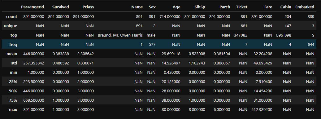
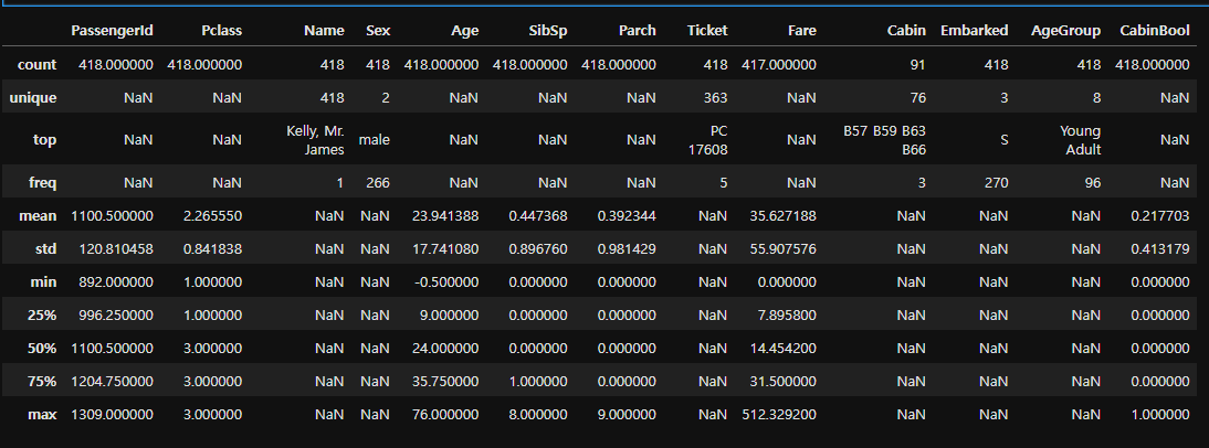
train.describe(include="all")

#get a list of the features within the dataset
print(train.columns)

train.info()
<class 'pandas.core.frame.DataFrame'>
RangeIndex: 891 entries, 0 to 890
Data columns (total 12 columns):

Column Non-Null Count Dtype

---

0 PassengerId 891 non-null int64
1 Survived 891 non-null int64
2 Pclass 891 non-null int64
3 Name 891 non-null object
4 Sex 891 non-null object
5 Age 714 non-null float64
6 SibSp 891 non-null int64
7 Parch 891 non-null int64
8 Ticket 891 non-null object
9 Fare 891 non-null float64
10 Cabin 204 non-null object
11 Embarked 889 non-null object
dtypes: float64(2), int64(5), object(5)
memory usage: 83.7+ KB

train.describe(include = "all")

#check for any other unusable values
print(pd.isnull(train).sum())

PassengerId 0
Survived 0
Pclass 0
Name 0
Sex 0
Age 177
SibSp 0
Parch 0
Ticket 0
Fare 0
Cabin 687
Embarked 2
dtype: int64

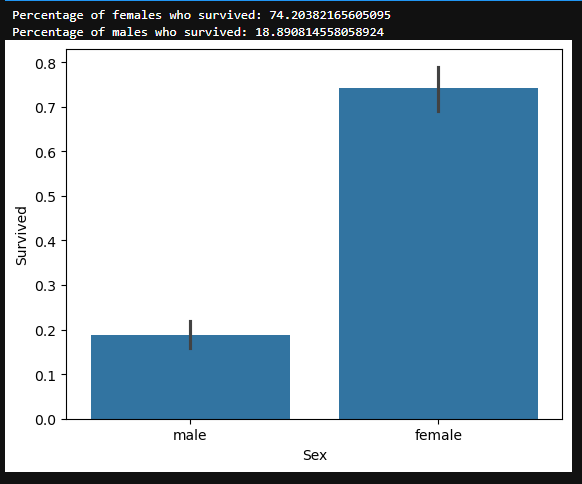
Sex Feature
#draw a bar plot of survival by sex
sns.barplot(x="Sex", y="Survived", data=train)

#print percentages of females vs. males that survive
print("Percentage of females who survived:", train["Survived"]train["Sex"] == 'female'].value_counts(normalize = True)[1]*100)

print("Percentage of males who survived:", train["Survived"]train["Sex"] == 'male'].value_counts(normalize = True)[1]*100)

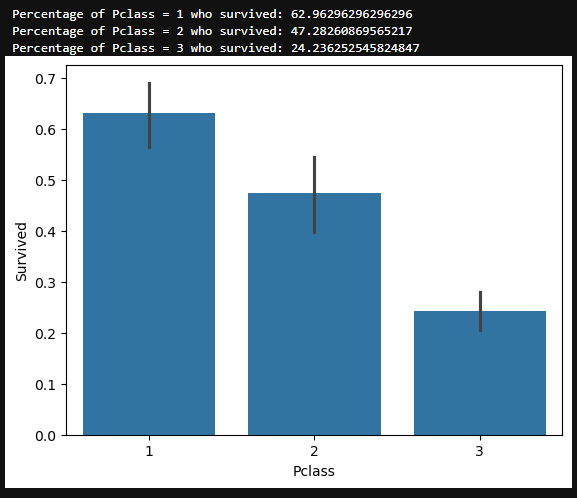
Pclass Feature¶
#draw a bar plot of survival by Pclass
sns.barplot(x="Pclass", y="Survived", data=train)

#print percentage of people by Pclass that survived
print("Percentage of Pclass = 1 who survived:", train["Survived"]train["Pclass"] == 1].value_counts(normalize = True)[1]*100)

print("Percentage of Pclass = 2 who survived:", train["Survived"]train["Pclass"] == 2].value_counts(normalize = True)[1]*100)

print("Percentage of Pclass = 3 who survived:", train["Survived"]train["Pclass"] == 3].value_counts(normalize = True)[1]*100)

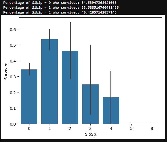
SibSp Feature¶
#draw a bar plot for SibSp vs. survival
sns.barplot(x="SibSp", y="Survived", data=train)

#I won't be printing individual percent values for all of these.
print("Percentage of SibSp = 0 who survived:", train["Survived"]train["SibSp"] == 0].value_counts(normalize = True)[1]*100)

print("Percentage of SibSp = 1 who survived:", train["Survived"]train["SibSp"] == 1].value_counts(normalize = True)[1]*100)

print("Percentage of SibSp = 2 who survived:", train["Survived"]train["SibSp"] == 2].value_counts(normalize = True)[1]*100)

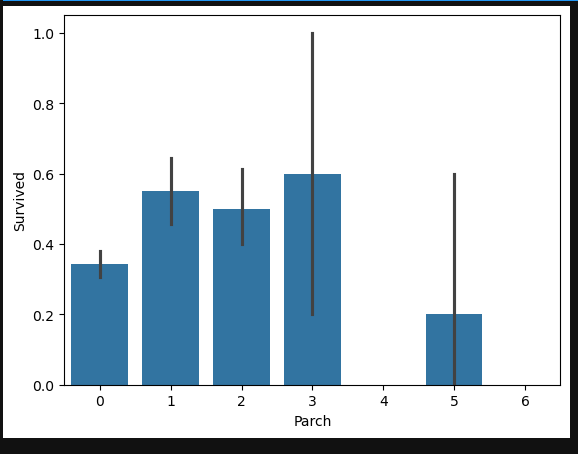
Parch Feature
#draw a bar plot for Parch vs. survival
sns.barplot(x="Parch", y="Survived", data=train)
plt.show()

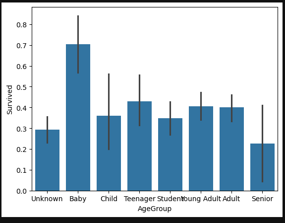
Age Feature
#sort the ages into logical categories
train["Age"] = train["Age"].fillna(-0.5)
test["Age"] = test["Age"].fillna(-0.5)
bins = [-1, 0, 5, 12, 18, 24, 35, 60, np.inf]
labels = ['Unknown', 'Baby', 'Child', 'Teenager', 'Student', 'Young Adult', 'Adult', 'Senior']
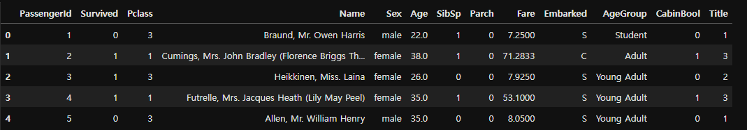
train['AgeGroup'] = pd.cut(train["Age"], bins, labels = labels)
test['AgeGroup'] = pd.cut(test["Age"], bins, labels = labels)

#draw a bar plot of Age vs. survival
sns.barplot(x="AgeGroup", y="Survived", data=train)
plt.show()

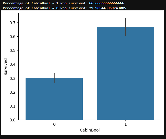
Cabin Feature
train["CabinBool"] = (train["Cabin"].notnull().astype('int'))
test["CabinBool"] = (test["Cabin"].notnull().astype('int'))

#calculate percentages of CabinBool vs. survived
print("Percentage of CabinBool = 1 who survived:", train["Survived"]train["CabinBool"] == 1].value_counts(normalize = True)[1]*100)

print("Percentage of CabinBool = 0 who survived:", train["Survived"]train["CabinBool"] == 0].value_counts(normalize = True)[1]*100)
#draw a bar plot of CabinBool vs. survival
sns.barplot(x="CabinBool", y="Survived", data=train)
plt.show()

test.describe(include="all")

Cabin Feature¶
#we'll start off by dropping the Cabin feature since not a lot more useful information can be extracted from it.
train = train.drop(['Cabin'], axis = 1)
test = test.drop(['Cabin'], axis = 1)

Ticket Feature
#we can also drop the Ticket feature since it's unlikely to yield any useful information
train = train.drop(['Ticket'], axis = 1)
test = test.drop(['Ticket'], axis = 1)

Embarked Feature
#now we need to fill in the missing values in the Embarked feature
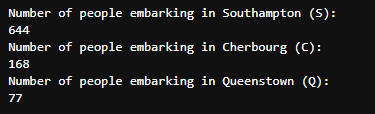
print("Number of people embarking in Southampton (S):")
southampton = train[train["Embarked"] == "S"].shape[0]
print(southampton)

print("Number of people embarking in Cherbourg (C):")
cherbourg = train[train["Embarked"] == "C"].shape[0]
print(cherbourg)

print("Number of people embarking in Queenstown (Q):")
queenstown = train[train["Embarked"] == "Q"].shape[0]
print(queenstown)

#replacing the missing values in the Embarked feature with S
train = train.fillna({"Embarked": "S"})

Age Feature¶
Next we'll fill in the missing values in the Age feature. Since a higher percentage of values are missing, it would be illogical to fill all of them with the same value (as we did with Embarked). Instead, let's try to find a way to predict the missing ages.

#create a combined group of both datasets
combine = [train, test]

#extract a title for each Name in the train and test datasets
for dataset in combine:
dataset['Title'] = dataset.Name.str.extract(' ([A-Za-z]+).', expand=False)

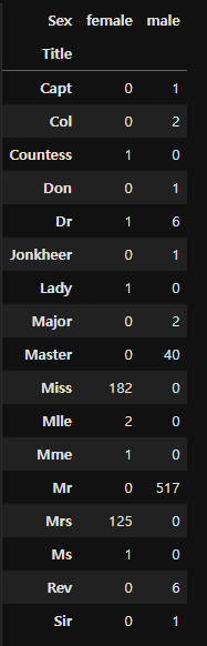
pd.crosstab(train['Title'], train['Sex'])

#replace various titles with more common names
for dataset in combine:
dataset['Title'] = dataset['Title'].replace(['Lady', 'Capt', 'Col',
'Don', 'Dr', 'Major', 'Rev', 'Jonkheer', 'Dona'], 'Rare')

dataset['Title'] = dataset['Title'].replace(['Countess', 'Lady', 'Sir'], 'Royal')
dataset['Title'] = dataset['Title'].replace('Mlle', 'Miss')
dataset['Title'] = dataset['Title'].replace('Ms', 'Miss')
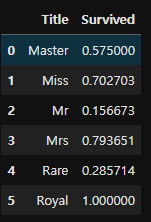
dataset['Title'] = dataset['Title'].replace('Mme', 'Mrs')

train[['Title', 'Survived']].groupby(['Title'], as_index=False).mean()

#map each of the title groups to a numerical value
title_mapping = {"Mr": 1, "Miss": 2, "Mrs": 3, "Master": 4, "Royal": 5, "Rare": 6}
for dataset in combine:
dataset['Title'] = dataset['Title'].map(title_mapping)
dataset['Title'] = dataset['Title'].fillna(0)

train.head()

fill missing age with mode age group for each title

mr_age = train[train["Title"] == 1]["AgeGroup"].mode() #Young Adult
miss_age = train[train["Title"] == 2]["AgeGroup"].mode() #Student
mrs_age = train[train["Title"] == 3]["AgeGroup"].mode() #Adult
master_age = train[train["Title"] == 4]["AgeGroup"].mode() #Baby
royal_age = train[train["Title"] == 5]["AgeGroup"].mode() #Adult
rare_age = train[train["Title"] == 6]["AgeGroup"].mode() #Adult

age_title_mapping = {1: "Young Adult", 2: "Student", 3: "Adult", 4: "Baby", 5: "Adult", 6: "Adult"}

#I tried to get this code to work with using .map(), but couldn't.
#I've put down a less elegant, temporary solution for now.
#train = train.fillna({"Age": train["Title"].map(age_title_mapping)})
#test = test.fillna({"Age": test["Title"].map(age_title_mapping)})

for x in range(len(train["AgeGroup"])):
if train["AgeGroup"][x] == "Unknown":
train["AgeGroup"][x] = age_title_mapping[train["Title"][x]]

for x in range(len(test["AgeGroup"])):
if test["AgeGroup"][x] == "Unknown":
test["AgeGroup"][x] = age_title_mapping[test["Title"][x]]

Now that we've filled in the missing values at least somewhat accurately (I will work on a better way for predicting missing age values), it's time to map each age group to a numerical value.

#map each Age value to a numerical value
age_mapping = {'Baby': 1, 'Child': 2, 'Teenager': 3, 'Student': 4, 'Young Adult': 5, 'Adult': 6, 'Senior': 7}
train['AgeGroup'] = train['AgeGroup'].map(age_mapping)
test['AgeGroup'] = test['AgeGroup'].map(age_mapping)

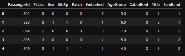
train.head()

#dropping the Age feature for now, might change
train = train.drop(['Age'], axis = 1)
test = test.drop(['Age'], axis = 1)

Name Feature
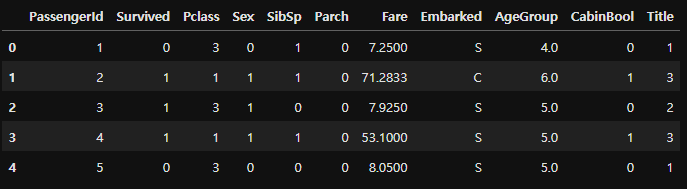
#drop the name feature since it contains no more useful information.
train = train.drop(['Name'], axis = 1)
test = test.drop(['Name'], axis = 1)

Sex Feature
#map each Sex value to a numerical value
sex_mapping = {"male": 0, "female": 1}
train['Sex'] = train['Sex'].map(sex_mapping)
test['Sex'] = test['Sex'].map(sex_mapping)

train.head()

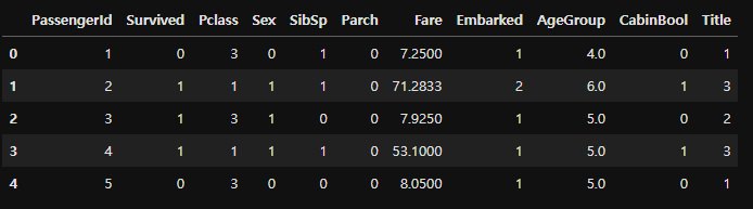
Embarked Feature
#map each Embarked value to a numerical value
embarked_mapping = {"S": 1, "C": 2, "Q": 3}
train['Embarked'] = train['Embarked'].map(embarked_mapping)
test['Embarked'] = test['Embarked'].map(embarked_mapping)

train.head()

Fare Feature
#fill in missing Fare value in test set based on mean fare for that Pclass
for x in range(len(test["Fare"])):
if pd.isnull(test["Fare"][x]):
pclass = test["Pclass"][x] #Pclass = 3
test["Fare"][x] = round(train[train["Pclass"] == pclass]["Fare"].mean(), 4)

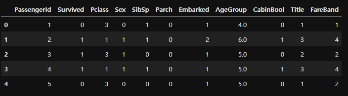
#map Fare values into groups of numerical values
train['FareBand'] = pd.qcut(train['Fare'], 4, labels = [1, 2, 3, 4])
test['FareBand'] = pd.qcut(test['Fare'], 4, labels = [1, 2, 3, 4])

#drop Fare values
train = train.drop(['Fare'], axis = 1)
test = test.drop(['Fare'], axis = 1)
#check train data
train.head()

#check test data
test.head()

Choosing the Best Model

Splitting the Training Data¶ We will use part of our training data (22% in this case) to test the accuracy of our different models.

from sklearn.model_selection import train_test_split

predictors = train.drop(['Survived', 'PassengerId'], axis=1)
target = train["Survived"]
x_train, x_val, y_train, y_val = train_test_split(predictors, target, test_size = 0.22, random_state = 0)

Testing Different Models¶ I will be testing the following models with my training data (got the list from here):

• Gaussian Naive Bayes
• Logistic Regression
• Support Vector Machines
• Perceptron
• Decision Tree Classifier
• Random Forest Classifier
• KNN or k-Nearest Neighbors
• Stochastic Gradient Descent
• Gradient Boosting Classifier For each model, we set the model, fit it with 80% of our training data, predict for 20% of the training data and check the accuracy.

Gaussian Naive Bayes

from sklearn.naive_bayes import GaussianNB
from sklearn.metrics import accuracy_score

gaussian = GaussianNB()
gaussian.fit(x_train, y_train)
y_pred = gaussian.predict(x_val)
acc_gaussian = round(accuracy_score(y_pred, y_val) * 100, 2)
print(acc_gaussian)

Logistic Regression

from sklearn.linear_model import LogisticRegression

logreg = LogisticRegression()
logreg.fit(x_train, y_train)
y_pred = logreg.predict(x_val)
acc_logreg = round(accuracy_score(y_pred, y_val) * 100, 2)
print(acc_logreg)

Support Vector Machines

from sklearn.svm import SVC

svc = SVC()
svc.fit(x_train, y_train)
y_pred = svc.predict(x_val)
acc_svc = round(accuracy_score(y_pred, y_val) * 100, 2)
print(acc_svc)

Linear SVC

from sklearn.svm import LinearSVC

linear_svc = LinearSVC()
linear_svc.fit(x_train, y_train)
y_pred = linear_svc.predict(x_val)
acc_linear_svc = round(accuracy_score(y_pred, y_val) * 100, 2)
print(acc_linear_svc)

Perceptron

from sklearn.linear_model import Perceptron

perceptron = Perceptron()
perceptron.fit(x_train, y_train)
y_pred = perceptron.predict(x_val)
acc_perceptron = round(accuracy_score(y_pred, y_val) * 100, 2)
print(acc_perceptron)

Decision Tree

from sklearn.tree import DecisionTreeClassifier

decisiontree = DecisionTreeClassifier()
decisiontree.fit(x_train, y_train)
y_pred = decisiontree.predict(x_val)
acc_decisiontree = round(accuracy_score(y_pred, y_val) * 100, 2)
print(acc_decisiontree)

Random Forest

from sklearn.ensemble import RandomForestClassifier

randomforest = RandomForestClassifier()
randomforest.fit(x_train, y_train)
y_pred = randomforest.predict(x_val)
acc_randomforest = round(accuracy_score(y_pred, y_val) * 100, 2)
print(acc_randomforest)

KNN or k-Nearest Neighbors

from sklearn.neighbors import KNeighborsClassifier

knn = KNeighborsClassifier()
knn.fit(x_train, y_train)
y_pred = knn.predict(x_val)
acc_knn = round(accuracy_score(y_pred, y_val) * 100, 2)
print(acc_knn)

Stochastic Gradient Descent

from sklearn.linear_model import SGDClassifier

sgd = SGDClassifier()
sgd.fit(x_train, y_train)
y_pred = sgd.predict(x_val)
acc_sgd = round(accuracy_score(y_pred, y_val) * 100, 2)
print(acc_sgd)

Gradient Boosting Classifier

from sklearn.ensemble import GradientBoostingClassifier

gbk = GradientBoostingClassifier()
gbk.fit(x_train, y_train)
y_pred = gbk.predict(x_val)
acc_gbk = round(accuracy_score(y_pred, y_val) * 100, 2)
print(acc_gbk)

models = pd.DataFrame({
'Model': ['Support Vector Machines', 'KNN', 'Logistic Regression',
'Random Forest', 'Naive Bayes', 'Perceptron', 'Linear SVC',
'Decision Tree', 'Stochastic Gradient Descent', 'Gradient Boosting Classifier'],
'Score': [acc_svc, acc_knn, acc_logreg,
acc_randomforest, acc_gaussian, acc_perceptron,acc_linear_svc, acc_decisiontree,
acc_sgd, acc_gbk]})
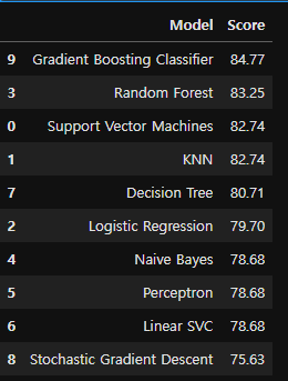
models.sort_values(by='Score', ascending=False)

Creating Submission File

It's time to create a submission.csv file to upload to the Kaggle competition!
#set ids as PassengerId and predict survival
ids = test['PassengerId']
predictions = gbk.predict(test.drop('PassengerId', axis=1))

#set the output as a dataframe and convert to csv file named submission.csv
output = pd.DataFrame({ 'PassengerId' : ids, 'Survived': predictions })
output.to_csv('submission.csv', index=False)

https://www.kaggle.com/code/nadintamer/titanic-survival-predictions-beginner