😃[3주차 - Day3]😃

4. Exploratory Data Analysis
탐색적 데이터 분석을 통해 데이터를 통달해봅시다. with Titanic Data
- 라이브러리 준비
- 분석의 목적과 변수 확인
- 데이터 전체적으로 살펴보기
- 데이터의 개별 속성 파악하기
0. 라이브러리 준비
import numpy as np
import pandas as pd
import matplotlib.pyplot as plt
import seaborn as sns

%matplotlib inline
tt_df = pd.read_csv("./train.csv")1. 분석의 목적과 변수 확인
tt_df.head(5)| PassengerId | Survived | Pclass | Name | Sex | Age | SibSp | Parch | Ticket | Fare | Cabin | Embarked | |
|---|---|---|---|---|---|---|---|---|---|---|---|---|
| 0 | 1 | 0 | 3 | Braund, Mr. Owen Harris | male | 22.0 | 1 | 0 | A/5 21171 | 7.2500 | NaN | S |
| 1 | 2 | 1 | 1 | Cumings, Mrs. John Bradley (Florence Briggs Th... | female | 38.0 | 1 | 0 | PC 17599 | 71.2833 | C85 | C |
| 2 | 3 | 1 | 3 | Heikkinen, Miss. Laina | female | 26.0 | 0 | 0 | STON/O2. 3101282 | 7.9250 | NaN | S |
| 3 | 4 | 1 | 1 | Futrelle, Mrs. Jacques Heath (Lily May Peel) | female | 35.0 | 1 | 0 | 113803 | 53.1000 | C123 | S |
| 4 | 5 | 0 | 3 | Allen, Mr. William Henry | male | 35.0 | 0 | 0 | 373450 | 8.0500 | NaN | S |
# 각 Coulum의 데이터 타입 확인하기

tt_df.dtypes
PassengerId int64
Survived int64
Pclass int64
Name object
Sex object
Age float64
SibSp int64
Parch int64
Ticket object
Fare float64
Cabin object
Embarked object
dtype: object2. 데이터 전체적으로 살펴보기
# 데이터 전체 정보를 얻는 함수 : .describe()

tt_df.describe() # 수치형 데이터에 대한 요약만을 제공합니다.| PassengerId | Survived | Pclass | Age | SibSp | Parch | Fare | |
|---|---|---|---|---|---|---|---|
| count | 891.000000 | 891.000000 | 891.000000 | 714.000000 | 891.000000 | 891.000000 | 891.000000 |
| mean | 446.000000 | 0.383838 | 2.308642 | 29.699118 | 0.523008 | 0.381594 | 32.204208 |
| std | 257.353842 | 0.486592 | 0.836071 | 14.526497 | 1.102743 | 0.806057 | 49.693429 |
| min | 1.000000 | 0.000000 | 1.000000 | 0.420000 | 0.000000 | 0.000000 | 0.000000 |
| 25% | 223.500000 | 0.000000 | 2.000000 | 20.125000 | 0.000000 | 0.000000 | 7.910400 |
| 50% | 446.000000 | 0.000000 | 3.000000 | 28.000000 | 0.000000 | 0.000000 | 14.454200 |
| 75% | 668.500000 | 1.000000 | 3.000000 | 38.000000 | 1.000000 | 0.000000 | 31.000000 |
| max | 891.000000 | 1.000000 | 3.000000 | 80.000000 | 8.000000 | 6.000000 | 512.329200 |
tt_df.corr()

# 인과성이 있다는 것은 아님. 높은 등급에 앉았다고 -> 생존한 확률이 올라간 것은 아님| PassengerId | Survived | Pclass | Age | SibSp | Parch | Fare | |
|---|---|---|---|---|---|---|---|
| PassengerId | 1.000000 | -0.005007 | -0.035144 | 0.036847 | -0.057527 | -0.001652 | 0.012658 |
| Survived | -0.005007 | 1.000000 | -0.338481 | -0.077221 | -0.035322 | 0.081629 | 0.257307 |
| Pclass | -0.035144 | -0.338481 | 1.000000 | -0.369226 | 0.083081 | 0.018443 | -0.549500 |
| Age | 0.036847 | -0.077221 | -0.369226 | 1.000000 | -0.308247 | -0.189119 | 0.096067 |
| SibSp | -0.057527 | -0.035322 | 0.083081 | -0.308247 | 1.000000 | 0.414838 | 0.159651 |
| Parch | -0.001652 | 0.081629 | 0.018443 | -0.189119 | 0.414838 | 1.000000 | 0.216225 |
| Fare | 0.012658 | 0.257307 | -0.549500 | 0.096067 | 0.159651 | 0.216225 | 1.000000 |
# 결측치를 확인합니다.

tt_df.isnull().sum()
PassengerId 0
Survived 0
Pclass 0
Name 0
Sex 0
Age 177
SibSp 0
Parch 0
Ticket 0
Fare 0
Cabin 687
Embarked 2
dtype: int643. 데이터의 개별 속성 파악하기
## 생존자, 사망자 명수는?

tt_df['Survived'].sum()342tt_df['Survived'].value_counts()0 549
1 342
Name: Survived, dtype: int64sns.countplot(x='Survived', data=tt_df)
plt.show()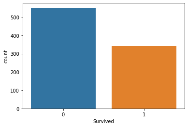
# Pclass에 따른 인원 파악

tt_df[['Pclass', 'Survived']].groupby(['Pclass']).count()| Survived | |
|---|---|
| Pclass | |
| 1 | 216 |
| 2 | 184 |
| 3 | 491 |
tt_df[['Pclass', 'Survived']].groupby(['Pclass']).sum()

# Survived가 1인 sum| Survived | |
|---|---|
| Pclass | |
| 1 | 136 |
| 2 | 87 |
| 3 | 119 |
tt_df_surv = tt_df[['Pclass', 'Survived']].groupby(['Pclass']).mean()

# 생존 비율
# 히트맵 사용 시각화
sns.heatmap(tt_df_surv)
plt.show()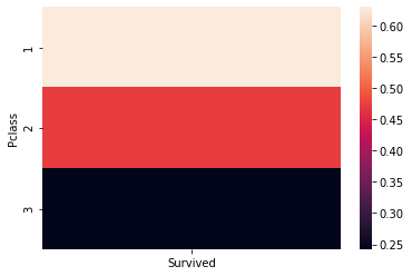
tt_df.groupby(['Survived', 'Sex'])['Survived'].count()Survived Sex
0 female 81
male 468
1 female 233
male 109
Name: Survived, dtype: int64sns.catplot(x='Sex', col='Survived', kind='count', data=tt_df)<seaborn.axisgrid.FacetGrid at 0x7f8d9c2b9ac8>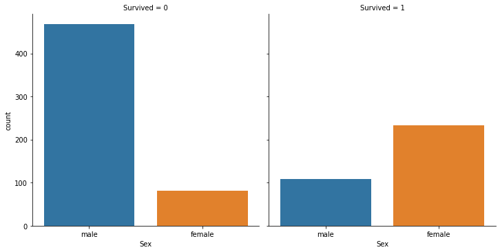
# 결측치가 존재하는 Age에 대해 분석을 합니다.

tt_df.describe()['Age']
count 714.000000
mean 29.699118
std 14.526497
min 0.420000
25% 20.125000
50% 28.000000
75% 38.000000
max 80.000000
Name: Age, dtype: float64fig, ax = plt.subplots(1,1, figsize=(10,5))
sns.kdeplot(x=tt_df[tt_df.Survived==1]['Age'], ax=ax)
sns.kdeplot(x=tt_df[tt_df.Survived==0]['Age'], ax=ax)
plt.legend(['Survived', 'Dead'])
plt.show()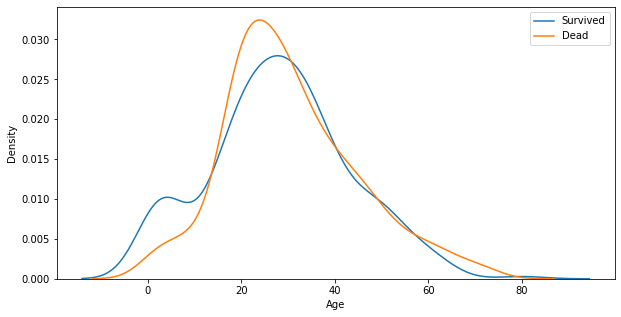
# Sex + Pclass vs Survived

sns.catplot(x='Pclass', y='Survived', hue='Sex', kind='point', data=tt_df)
plt.show()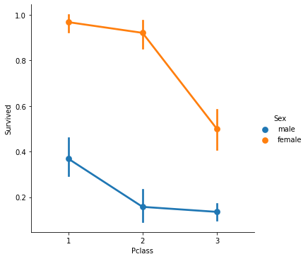
# Age + Pclass

tt_df['Age'][tt_df.Pclass == 1].plot(kind='kde')
tt_df['Age'][tt_df.Pclass == 2].plot(kind='kde')
tt_df['Age'][tt_df.Pclass == 3].plot(kind='kde')

plt.legend(['1st','2nd','3rd'])
plt.show()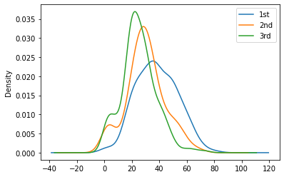
Mission : It's Your Turn!
1. 본문에서 언급된 Feature를 제외하고 유의미한 Feature를 1개 이상 찾아봅시다.
- Hint : Fare? Sibsp? Parch?
2. Kaggle에서 Dataset을 찾고, 이 Dataset에서 유의미한 Feature를 3개 이상 찾고 이를 시각화해봅시다.
함께 보면 좋은 라이브러리 document
무대뽀로 하기 힘들다면? 다음 Hint와 함께 시도해봅시다:
- 데이터를 톺아봅시다.
- 각 데이터는 어떤 자료형을 가지고 있나요?
- 데이터에 결측치는 없나요? -> 있다면 이를 어떻게 메꿔줄까요?
- 데이터의 자료형을 바꿔줄 필요가 있나요? -> 범주형의 One-hot encoding
- 데이터에 대한 가설을 세워봅시다.
- 가설은 개인의 경험에 의해서 도출되어도 상관이 없습니다.
- 가설은 명확할 수록 좋습니다 ex) Titanic Data에서 Survival 여부와 성별에는 상관관계가 있다!
- 가설을 검증하기 위한 증거를 찾아봅시다.
- 이 증거는 한 눈에 보이지 않을 수 있습니다. 우리가 다룬 여러 Technique를 써줘야합니다.
.groupby()를 통해서 그룹화된 정보에 통계량을 도입하면 어떨까요?.merge()를 통해서 두개 이상의 dataFrame을 합치면 어떨까요?- 시각화를 통해 일목요연하게 보여주면 더욱 좋겠죠?
Mission : It's Your Turn!
1. 본문에서 언급된 Feature를 제외하고 유의미한 Feature를 1개 이상 찾아봅시다.
- Hint : Fare? Sibsp? Parch?
# 1등석, 2등석, 3등석과 승선한 위치의 상관관계? (승객의 지위, 부유한 지역 판단하기)

Pclass1 = tt_df[tt_df['Embarked']=='S']['Pclass'].value_counts()
Pclass2 = tt_df[tt_df['Embarked']=='C']['Pclass'].value_counts()
Pclass3 = tt_df[tt_df['Embarked']=='Q']['Pclass'].value_counts()

S_people = tt_df[tt_df['Embarked']=='S']['PassengerId'].count()
C_people = tt_df[tt_df['Embarked']=='C']['PassengerId'].count()
Q_people = tt_df[tt_df['Embarked']=='Q']['PassengerId'].count()

df = pd.DataFrame([Pclass1 / S_people, Pclass2 / C_people, Pclass3 / Q_people])
df.index = ['S', 'C', 'Q']

df.plot(kind='bar')
plt.show()

# Q 지역은 3등석의 비율이 제일 높고 1등석의 비율은 C지역이 제일 높습니다.
# 클래스와 생존률의 상관관계? (그렇다면 부의 척도가, 생존률에도 영향을 미치는가)

sns.countplot(data=tt_df, x='Pclass', hue='Survived')
plt.show()

# 질문 1. 이 플롯과 요 바로 위 플롯을 합쳐서 표현하고 싶을 때, 어떻게 그려야하는지!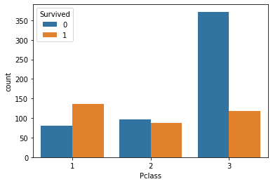
# 승선한 지역과 클래스간의 플롯 (S가 제일 많이 승선했고, Q는 3등석에 몰려있다.)

tt_df.groupby(['Embarked','Pclass'])['PassengerId'].count().plot(kind="bar")
plt.xticks(rotation=0)
plt.show()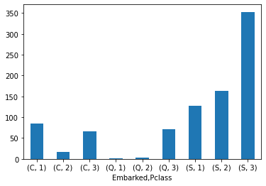
2. Kaggle에서 Dataset을 찾고, 이 Dataset에서 유의미한 Feature를 3개 이상 찾고 이를 시각화해봅시다.
함께 보면 좋은 라이브러리 document
Netflix Movies and TV Shows 에 대한 데이터를 가지고 진행하였습니다.
netflix = pd.read_csv("./netflix_titles.csv")

netflix.tail(5)| show_id | type | title | director | cast | country | date_added | release_year | rating | duration | listed_in | description | |
|---|---|---|---|---|---|---|---|---|---|---|---|---|
| 6229 | 80000063 | TV Show | Red vs. Blue | NaN | Burnie Burns, Jason Saldaña, Gustavo Sorola, G... | United States | NaN | 2015 | NR | 13 Seasons | TV Action & Adventure, TV Comedies, TV Sci-Fi ... | This parody of first-person shooter games, mil... |
| 6230 | 70286564 | TV Show | Maron | NaN | Marc Maron, Judd Hirsch, Josh Brener, Nora Zeh... | United States | NaN | 2016 | TV-MA | 4 Seasons | TV Comedies | Marc Maron stars as Marc Maron, who interviews... |
| 6231 | 80116008 | Movie | Little Baby Bum: Nursery Rhyme Friends | NaN | NaN | NaN | NaN | 2016 | NaN | 60 min | Movies | Nursery rhymes and original music for children... |
| 6232 | 70281022 | TV Show | A Young Doctor's Notebook and Other Stories | NaN | Daniel Radcliffe, Jon Hamm, Adam Godley, Chris... | United Kingdom | NaN | 2013 | TV-MA | 2 Seasons | British TV Shows, TV Comedies, TV Dramas | Set during the Russian Revolution, this comic ... |
| 6233 | 70153404 | TV Show | Friends | NaN | Jennifer Aniston, Courteney Cox, Lisa Kudrow, ... | United States | NaN | 2003 | TV-14 | 10 Seasons | Classic & Cult TV, TV Comedies | This hit sitcom follows the merry misadventure... |
netflix.info()<class 'pandas.core.frame.DataFrame'>
RangeIndex: 6234 entries, 0 to 6233
Data columns (total 12 columns):
# Column Non-Null Count Dtype
--- ------ -------------- -----
0 show_id 6234 non-null int64
1 type 6234 non-null object
2 title 6234 non-null object
3 director 4265 non-null object
4 cast 5664 non-null object
5 country 5758 non-null object
6 date_added 6223 non-null object
7 release_year 6234 non-null int64
8 rating 6224 non-null object
9 duration 6234 non-null object
10 listed_in 6234 non-null object
11 description 6234 non-null object
dtypes: int64(2), object(10)
memory usage: 584.6+ KBnetflix.nunique()show_id 6234
type 2
title 6172
director 3301
cast 5469
country 554
date_added 1524
release_year 72
rating 14
duration 201
listed_in 461
description 6226
dtype: int641. 넷플릭스에는 최근에 나온 영화 및 TV쇼가 많이 등록되어 있을까 아니면 옛날 영화가 많을까에 대한 추론을 해보았습니다.
fig, ax = plt.subplots(figsize=(15,10))
sns.countplot(ax = ax, data = netflix, x = 'release_year', hue="type")
plt.legend(loc='center')
plt.xticks(rotation='70')
plt.show()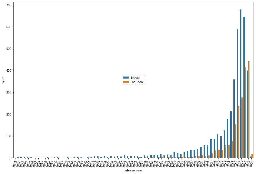
아마존의 심의등급은 아래와 같습니다.
ratings_data = { 'TV-PG': 7,'TV-MA': 18,'TV-Y7-FV': 7,'TV-Y7': 7,
            'TV-14': 16,'R': 18,'TV-Y': 0,'NR': 18,'PG-13': 13,
            'TV-G': 0,'PG': 7,'G': 0,'UR': 18,'NC-17': 18}

ratings = pd.Series(ratings_data, name='recommand_age')
ratings
TV-PG 7
TV-MA 18
TV-Y7-FV 7
TV-Y7 7
TV-14 16
R 18
TV-Y 0
NR 18
PG-13 13
TV-G 0
PG 7
G 0
UR 18
NC-17 18
Name: recommand_age, dtype: int64netflix = pd.merge(netflix, ratings, left_on='rating', right_index=True)
netflix.head()| show_id | type | title | director | cast | country | date_added | release_year | rating | duration | listed_in | description | recommand_age | |
|---|---|---|---|---|---|---|---|---|---|---|---|---|---|
| 0 | 81145628 | Movie | Norm of the North: King Sized Adventure | Richard Finn, Tim Maltby | Alan Marriott, Andrew Toth, Brian Dobson, Cole... | United States, India, South Korea, China | September 9, 2019 | 2019 | TV-PG | 90 min | Children & Family Movies, Comedies | Before planning an awesome wedding for his gra... | 7 |
| 30 | 80988892 | Movie | Next Gen | Kevin R. Adams, Joe Ksander | John Krasinski, Charlyne Yi, Jason Sudeikis, M... | China, Canada, United States | September 7, 2018 | 2018 | TV-PG | 106 min | Children & Family Movies, Comedies, Sci-Fi & F... | When lonely Mai forms an unlikely bond with a ... | 7 |
| 43 | 80095641 | Movie | Elstree 1976 | Jon Spira | Paul Blake, Jeremy Bulloch, John Chapman, Anth... | United Kingdom | September 6, 2016 | 2015 | TV-PG | 102 min | Documentaries | Then and now footage of bit players who appear... | 7 |
| 48 | 81016045 | Movie | One Day | Banjong Pisanthanakun | Chantavit Dhanasevi, Nittha Jirayungyurn, Thee... | Thailand | September 5, 2018 | 2016 | TV-PG | 135 min | Dramas, International Movies, Romantic Movies | When his colleague (and crush) temporarily los... | 7 |
| 67 | 80128317 | TV Show | The Eighties | NaN | NaN | United States | September 30, 2018 | 2016 | TV-PG | 1 Season | Docuseries | This nostalgic documentary series relives the ... | 7 |
2. 어린이를 위한 영화 및 TV 쇼는 얼마나 존재할지, 얼마나 키즈-프렌들리한 어플리케이션일지 알아보겠습니다.
data_by_age = netflix.groupby(["recommand_age",'type'])['show_id'].count()

data_by_age.plot.pie(figsize=(15,10))
plt.show()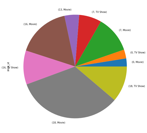
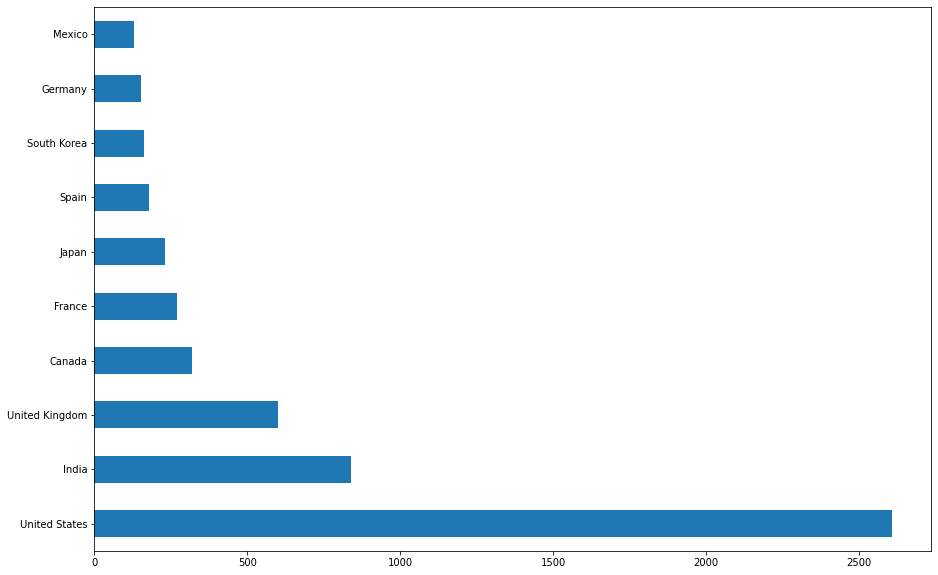
3. 어느지역이 제일 많은 영상을 보유하고 있는가?
import collections as c

country_count = c.Counter(", ".join(netflix['country'].dropna()).split(", "))
top_ten_countries = country_count.most_common(10)
rank = {}
for x in top_ten_countries:
  rank[x[0]] = x[1]
rank_series = pd.Series(rank)

rank_series.plot(kind='barh', figsize=(15,10))
plt.show()