1. MNIST 손글씨 분류
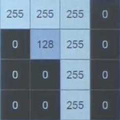
손글씨의 경우 픽셀 값으로 분류할 수 있다. 해당 한 칸은 1byte이며, 1~255까지의 숫자를 포함한다. 예를 들어 7의 경우에는 아래와 같이 나타낼 수 있다.
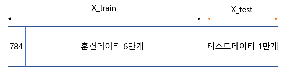
학습을 위해서는 데이터셋의 구성을 잘 알필요가 있다. 아래와 같이 reshape를 사용해서 데이터를 잘라주며, x_train에는 6만개의 데이터셋을, x_test에는 1만개의 데이터셋을 넣어준다. 아래의 코드에서 astype으로 float형을 만든 다음, 255로 나눠주면 모든 byte가 0~1사이의 실수가 된다. 이것이 정규화 과정이다.

여기서 손글씨에 사용되는 글자는 모두 28*28 사이즈이므로 784byte가 나오게 된다. 이것을 정리한다면 아래와 같이 나타낼 수 있다.
모델 훈련 fit(train, batch_size, epochs)
1. batch_size
batch size는 계산 중간의 갱신 값이다. 예를들어, 100문제가 있고, batch size=100이면, 1번의 갱신이 일어난다. 만약 100문제 batch size=10이라면 10문제 풀 때마다 갱신되어 총 10번의 갱신이 일어난다.
즉, batch size는 적을수록 답을 많이 갱신하여 정답률이 높아지지만, 많은 연산으로 인해 메모리 소모가 많아진다.
2. epochs
epochs는 반복횟수로 늘어날 수록 정답률이 높아지지만, 처음으로 관측되는 데이터가 있을 때는 정답률이 떨어지게 된다. 이것을 overfitting(과적합)이라 한다.
3. 훈련 예시
여기서는 수능 문제 훈련을 예시로 들었다. 만약 올해 수능문제를 예측으로 둔다면 훈련셋으로 하나를 제외한 모의고사 전체를, 검증셋으로 제외됐던 모의고사를, 시험셋으로 작년 수능문제를 둔다.
즉, 예측 = 훈련 + 검증 + 시험셋 이다.
softmax
softmax는 다중 분류 함수이다. 모든 분류의 합 값이 1이 되어야한다.
예를 들어, 삼각형, 사각형, 원이 있을 때 분류값이 각각 0.1,0.2,0.7이 되어야 한다는 것이다. 수식적인 부분은 전 포스팅에 있으므로 참고.
모델 구성하기
모델 구성은 보통 Sequential()로 한다.
model = Sequential()
model.add(Dense(output_dim=64, input_dim=28*28, activation='relu'))
model.add(Dense(ouput_dim=10, activation='softmax'))
라는 코드가 있을 때, 첫 입력층에서는 input의 크기를 적어줘야 한다. 또한 'relu'라는 경사함수로 처리한다. (relu는 max(0,input) 값으로 경사함수가 된다.)
두번째 은닉층에서는 output_dim=10인데, 0~9까지 10개의 숫자로 분류하기 때문이다. 또한 softmax를 통한 다중 클래스 분류를 행한다.
전체 코드
#0. 사용할 패키지 불러오기
from keras.utils import np_utils
from keras.datasets import mnist
from keras.models import Sequential
from keras.layers import Dense, Activation

#1. 데이터셋 생성하기
(x_train, y_train), (x_test, y_test) = mnist.load_data()
x_train = x_train.reshape(60000, 784).astype('float32') / 255.0
x_test = x_test.reshape(10000, 784).astype('float32') / 255.0
y_train = np_utils.to_categorical(y_train)
y_test = np_utils.to_categorical(y_test)

#2. 모델 구성하기
model = Sequential()
model.add(Dense(units=64, input_dim=28*28, activation='relu'))
model.add(Dense(units=10, activation='softmax'))

#3. 모델 학습과정 설정하기
model.compile(loss='categorical_crossentropy', optimizer='sgd', metrics=['accuracy'])

#4. 모델 학습시키기
hist = model.fit(x_train, y_train, epochs=5, batch_size=32)

#5. 학습과정 살펴보기
print('## training loss and acc ##')
print(hist.history['loss'])
print(hist.history['accuracy'])

#6. 모델 평가하기
loss_and_metrics = model.evaluate(x_test, y_test, batch_size=32)
print('## evaluation loss and_metrics ##')
print(loss_and_metrics)

#7. 모델 사용하기
xhat = x_test[0:1]
yhat = model.predict(xhat)
print('## yhat ##')
print(yhat)