GAN(Generative Adversarial Nets)

Yann LeCun(Director, Meta AI) described GANs as “the most interesting idea in the last 10 years in Machine Learning.”

Today, I'll introduce this remarkable generative model.

1. Overview

Before diving into what GAN is, I’d like to give a brief introduction what GAN can do.

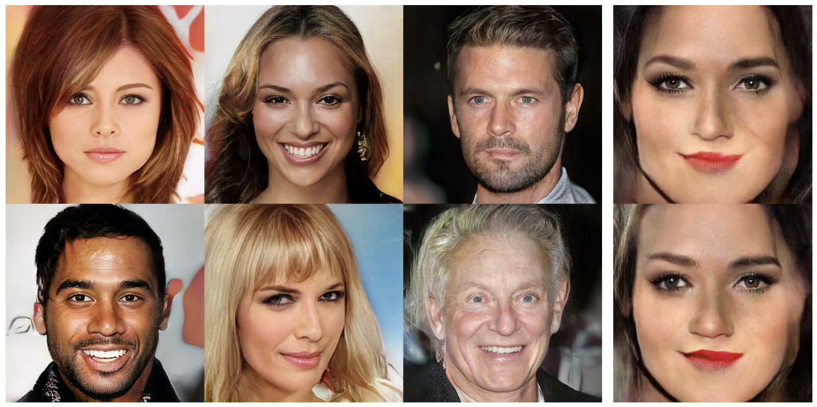
All the images you see here are synthetic faces created by GANs (StyleGAN2).

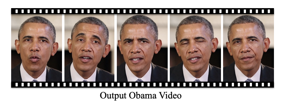
Also, GAN can generate fake videos
link: https://www.youtube.com/watch?v=AmUC4m6w1wo

even transform photos of closed eyes into photos the person’s eyes are open.

In this post, we will take a look at basic GAN model, the predecessor of these various GAN models, including simple adversarial net training example and mathematical proof.

2. Background and Problem Definition

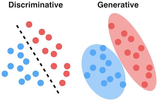
Generative model

Produce an image that does not exist but is likely to exist

• A statistical model of the joint probability distribution

• An architecture to generate new data instances
  

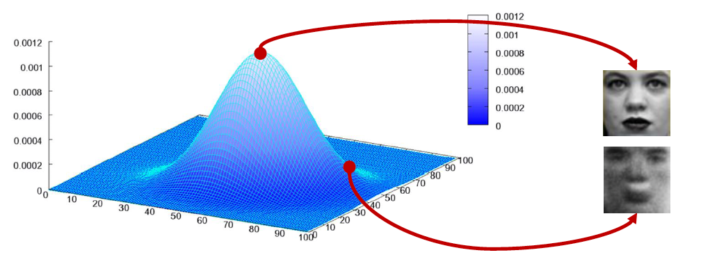
• The goal of a generative model is to create a model $G$ that approximates the distribution of image data

• Model $G$ works well means It can model the distribution of original images well

  • A representative example is Generative Adversarial Networks(GAN), proposed in 2014
  • Many papers have stemmed from GAN

Problem Definition

• The GAN framework pits two adversaries against each other in a dynamic interplay. Each model is represented by a differentiable function controlled by a set of parameters.
• Typically these functions are implemented as deep neural networks. The interplay proceeds in two scenarios.
  1. In first scenario, The discriminator $D$learns to distinguish between real data samples and the fake samples produced by $G$. It is trained to maximize its ability to correctly classify real and generated data. In this first scenario, the goal of the discriminator is for $D(x)$ to be near $1$.
  2. In the second scenario, The generator $G$ learns to produce samples that mimic real data, drawing from a random input (noise) to approximate the distribution of actual data, $p_{data}$. In this scenario, both models participate. The discriminator strives to make $D(G(z))$ approach $0$ while the generative strives to make the same quantity approach $1$.
• If both models have sufficient capacity, then the Nash equilibrium of this framework corresponds to the $G(z)$ being drawn from the same distribution as the training data, and $D(x)$ = $1\over2$ for all $x$.

  Nash Equilibrium: situation where no model could gain by changing their own strategy (holding all other model's strategies fixed)

3. Main Method

Adversarial Nets

Based on the concepts discussed in the problem definition, let’s examine the structure of how the actual neural network is implemented.

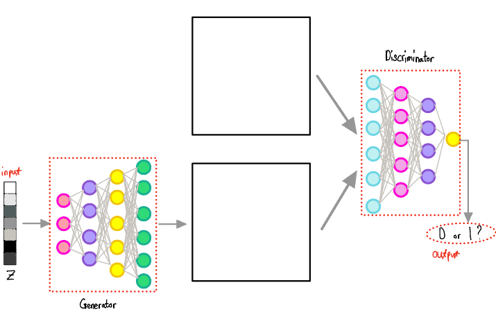
• As you can see the input is 1 dimensional vector, and the output is a number between 0 and 1.
• The part that takes a 1-dimensional vector as input acts as fake, the generator
• The part that outputs either 0 or 1 is the discriminator which plays the role of an appraiser identifying forgeries.

As the fake created imitations, let's assume that we have a neural network that takes a random 1-dimensional vector as input to generate a human face.

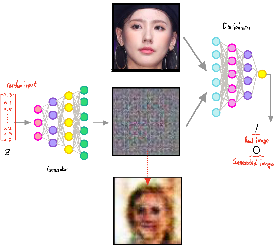
• Since the weights of Generator's neural network are random at the begining and the input is always random, the generator would make hard to recongnize output at first.
• Discriminator prepares the real data for training
• Then, one of these two is used as input of the Discriminator
• The point here is that one of the inputs is randomly selected. From the Discriminator's view, it doesn't know whether the incoming input is a generated photo or a real photo. It must rely on the data, like an appraiser, to distinguish whether the input is real or not.
• Therefore in the case of Discriminator, it should be trained to output a value close to 1 when the real image is input. When a fake image is input, it should be trained to produce an ouput close to 0.
• As the Discriminator improves, the generator is also trained to produce images which resemble real images more closely

Learning process resembles a competitive between models, this model is called Generative Adversarial Network.

Theoretical Results: Proof of Global optimality

Proof of convergence $p_g$ to $p_{data}$

The theoretical results are divided into two main parts:

1. Demonstrate that the previously introduced minimax problem has a global optimum when $p_g = p_{data}$
2. Then show that the algorithm proposed in this paper can reach this global optimum.
   

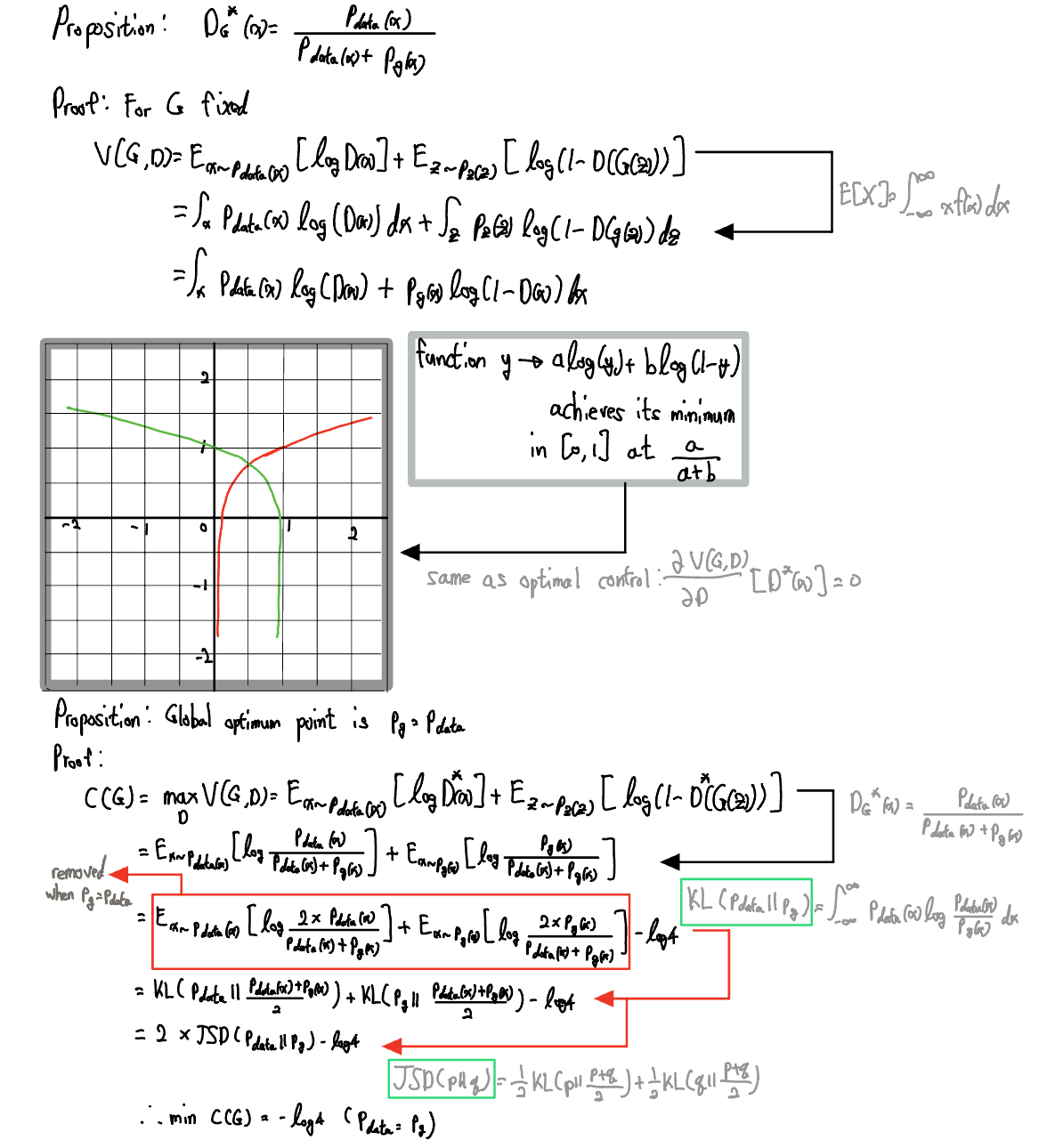
• KL(KullBack Leibler) Divergence: A formula that quantitatively expresses how much two distributions differ from each other. In practice, it’s often adjusted more for the sake of convenience in proofs.
  link: https://en.wikipedia.org/wiki/Kullback%E2%80%93Leibler_divergence
  In the case of KL Divergence, it is difficult to use as distance metric
  => Use Jensen-Shannon Divergence
• Jensen-Shannon Divergence: Used to measure the distance between two distributions. As a distance metric, it has a minimum value of 0 when $p_{data} = p_g$
  link: https://en.wikipedia.org/wiki/Jensen%E2%80%93Shannon_divergence
• The generator reaches a global optimal point when the images it outputs match the original data distribution. Therefore, if the generator is well-trained after the discriminator has already converged, it can converge to a distribution similar to $p_{data}$

Now, let’s take a closer look at how the GAN model processes information and learns, using actual numbers for a simple example.

Actual neural network implementation

Since we are calculating with actual numbers, I will use the simplest model possible.

1. Forward Propagation
   

• Each generator and discriminator will be constructed as single-layer neural networks for simplicity in calculations.
• The input will be a value of size 1, which lies between 0 and 1($z$ is set to $0.5$ here).
• This input will be calculated with the weights of the generator to create a $1$-dimensional matrix with three elements, essentially producing an RGB matrix ($3 \times 1$). For the real data part, we will define the RGB value for pure red.
• The goal of training is to have the generator output RGB value close to pure red ($0.99, 0.01, 0.01$).
• It is expressed the value between 0 and 1 through the calculations and sigmoid function, and forward-propagate as follows.
• Bias should be included for complete generator and discriminator, we will omit for the simplicity.

Let's examine how errors originating from the loss function propagate backward.

2. Back Propagation
   

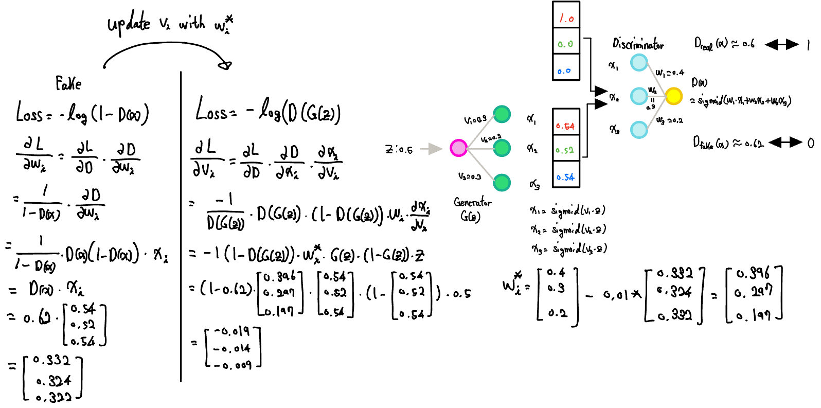
• With chain rule, the weight of discriminator $w^*$ is updated(when learning rate = 0.01)
• After updating the weights of the discriminator, we use those weights to train the generator.
• We can update in the weight of the generator as follows.

4. Results and Analysis

Visualization of Experiment

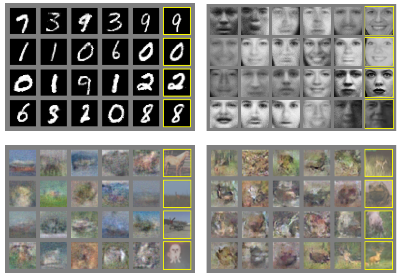
Figure: Visualization of samples from the model

• Not cherry-picked
• Not memorized the training set: As shown in yellow box(training data) and non-yellow box(generated data)
• Competitive with the better generative models
• Images represent sharp(compared with autoencoder based generative models)
  
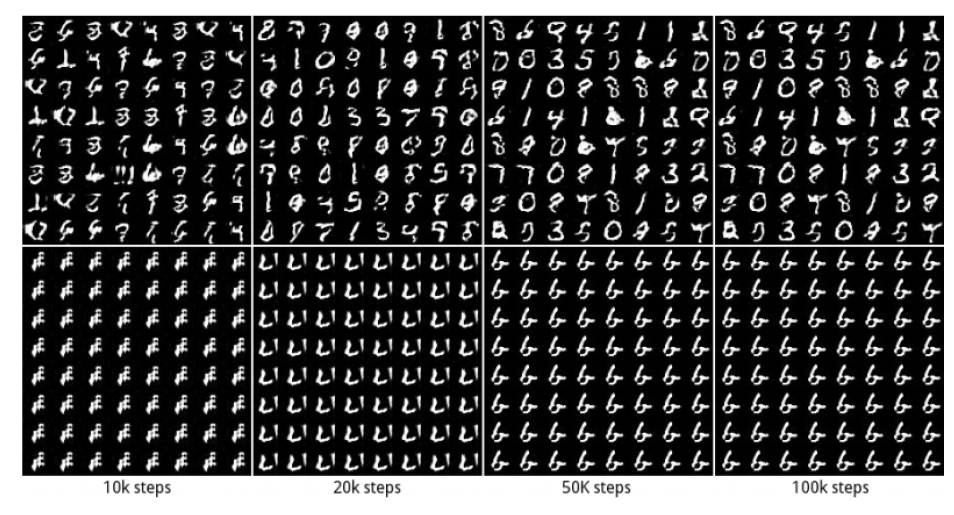
  Figure: Digits obtained by linearly interpolating between coordinates in $z$ space of the model

5. Advantages and Limitations

Advantages

• Computational efficiency: Markov chains are not needed, and only backpropagation is used to obtain gradients.
• Flexibility: a wide variety of functions can be incorporated into the model.
• Statistical advantage: The generator network is updated only with gradients flowing through the discriminator, not directly with data samples, meaning that components of the input are not copied directly into the generator's parameters.
• Sharp Distributions: As shown above experiment part, GANs can represent very sharp, even degenerate distributions, whereas Markov chain-based methods require the distribution to be somewhat blurry to facilitate mixing between modes.

Markov chain: Stochastic process describing a sequence of possible events in which the probability of each event depends only on the state attained in the previous event. It has limitation for blurred distribution and computational loss for negative chain updating process.
More: https://en.wikipedia.org/wiki/Markov_chain

Limitations

• One critical drawback of GANs is their highly unstable training process. Since there is no explicit representation of the data distribution $p_g(x)$ that the Generator approximates, balancing the training of G and D becomes challenging.

• This instability often leads to model collapse, or the Helvetica scenario. If the Generator G trains much faster than the Discriminator $D$, $G$ may focus on specific data points that easily deceive $D$, resulting in the generation of similar samples. In latent space, different $z$ values get mapped to similar outputs.

• Model collapse happens because the Generator's objective is to fool the Discriminator rather than produce diverse, high-quality data. Thus, while generative models are expected to create varied outputs, GANs often fail to do so since the $V(G,D)$ objective lacks a diversity-promoting term.

• Partial mode collapse is more common than complete mode collapse, where the Generator focuses on data around a specific target point. This local minimum problem arises because once $D$ is deceived, it struggles to regain its discrimination ability, shifting the min-max in favor of the Generator.
  
  Model-collapse example image

Some effective techniques currently known to address mode collapse include:

• Feature matching : Adding a least square error term between fake and real data to the loss function.
• Mini batch discrimination : Including the sum of differences between fake and real data across mini-batches in the loss function.
• Historical averaging : Incorporating previous batch updates to retain the impact of past training information as a way to guide learning.

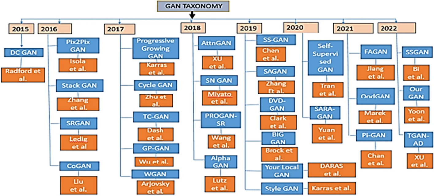
Despite these drawbacks, the significant advantages of GANs have led to the development of numerous variations. (Refer to the GAN hierarchy image from an overview.)

6. Quick Summary and Concluding the Posting

I have covered what GAN can do, Background, Main method, experiment and its advantage and limitations. I hope my detailed and simple explanation of GAN helps you understand this model better!

For my first blog post, I chose to cover the well-known generative model paper GAN. The detailed and clear explanations of the formulas in the paper made it easy to write and expand upon in my post, and following the flow helped the concepts really sink in. This experience reinforced the idea that true knowledge comes from not only absorbing but also expressing and explaining it. Figuring out my understanding of the model and explaining the equations improved my comprehension significantly. I’d like to try a personal project using GANs to implement the concepts in code. If I continue studying AI research papers, I’ll aim to post regularly on this blog as a way to track my learning journey.

References were noted in the comments due to content restrictions issue