데이터소개
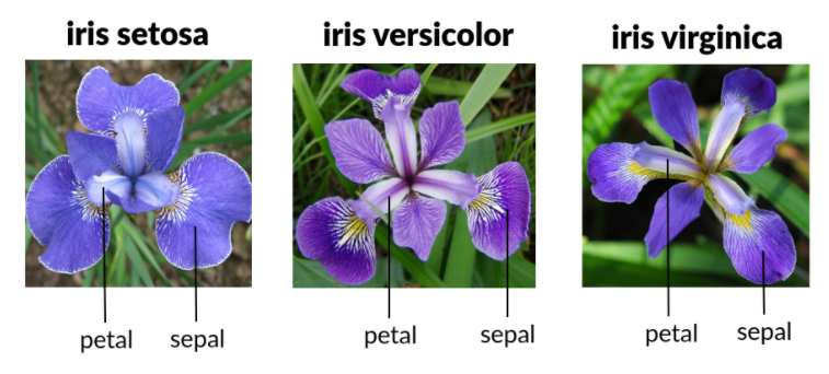
iris는 Setosa, Versicolour, Virginica의 3가지 종류의 꽃에 대해서 꽃잎(petal)과 꽃받침(sepal)의 길이(length)와 너비(width)를 나타낸 데이터이다. iris 데이터에서 특징을 이용해 꽃의 종류를 구별할 수 있다.
데이터분석
- 꽃의 종류을 구별
Setosa, Versicolour, Virginica
iris.target_names -> Setosa, Versicolour, Virginica- 꽃의 특징을 구별
꽃받침의 길이와 넓이, 꽃잎의 길이와 넓이로 총 4가지
iris.feature_names -> sepal length, sepal width, petal length, petal width- 총 데이터의 개수와 dim
dimension을 나타내는 d=4, 총 데이터의 개수는 n=150
iris.data -> n(=150)-by-4 data arrays아래와 같이 전체 데이터는 4 column데이터가 된다.
{'data': array([[5.1, 3.5, 1.4, 0.2],
       [4.9, 3. , 1.4, 0.2],
       [4.7, 3.2, 1.3, 0.2],
       [4.6, 3.1, 1.5, 0.2],
       [5. , 3.6, 1.4, 0.2],
       [5.4, 3.9, 1.7, 0.4],
       [4.6, 3.4, 1.4, 0.3],
       [5. , 3.4, 1.5, 0.2],
       [4.4, 2.9, 1.4, 0.2],
       .
       .(길어서 생략함)
       .
       [5.8, 2.7, 5.1, 1.9],
       [6.8, 3.2, 5.9, 2.3],
       [6.7, 3.3, 5.7, 2.5],
       [6.7, 3. , 5.2, 2.3],
       [6.3, 2.5, 5. , 1.9],
       [6.5, 3. , 5.2, 2. ],
       [6.2, 3.4, 5.4, 2.3],
       [5.9, 3. , 5.1, 1.8]]), 'target': array([0, 0, 0, 0, 0, 0, 0, 0, 0, 0, 0, 0, 0, 0, 0, 0, 0, 0, 0, 0, 0, 0,
       0, 0, 0, 0, 0, 0, 0, 0, 0, 0, 0, 0, 0, 0, 0, 0, 0, 0, 0, 0, 0, 0,
       0, 0, 0, 0, 0, 0, 1, 1, 1, 1, 1, 1, 1, 1, 1, 1, 1, 1, 1, 1, 1, 1,
       1, 1, 1, 1, 1, 1, 1, 1, 1, 1, 1, 1, 1, 1, 1, 1, 1, 1, 1, 1, 1, 1,
       1, 1, 1, 1, 1, 1, 1, 1, 1, 1, 1, 1, 2, 2, 2, 2, 2, 2, 2, 2, 2, 2,
       2, 2, 2, 2, 2, 2, 2, 2, 2, 2, 2, 2, 2, 2, 2, 2, 2, 2, 2, 2, 2, 2,
       2, 2, 2, 2, 2, 2, 2, 2, 2, 2, 2, 2, 2, 2, 2, 2, 2, 2]), 'frame': None, 'target_names': array(['setosa', 'versicolor', 'virginica'], dtype='<U10'), 'DESCR': '.. _iris_dataset:\n\nIris plants dataset\n--------------------\n\n**Data Set Characteristics:**\n\n    :Number of Instances: 150 (50 in each of three classes)\n    :Number of Attributes: 4 numeric, predictive attributes and the class\n    :Attribute Information:\n        - sepal length in cm\n        - sepal width in cm\n        - petal length in cm\n        - petal width in cm\n        - class:\n                - Iris-Setosa\n                - Iris-Versicolour\n                - Iris-Virginica\n                \n    :Summary Statistics:\n\n    ============== ==== ==== ======= ===== ====================\n                    Min  Max   Mean    SD   Class Correlation\n    ============== ==== ==== ======= ===== ====================\n    sepal length:   4.3  7.9   5.84   0.83    0.7826\n    sepal width:    2.0  4.4   3.05   0.43   -0.4194\n    petal length:   1.0  6.9   3.76   1.76    0.9490  (high!)\n    petal width:    0.1  2.5   1.20   0.76    0.9565  (high!)\n    ============== ==== ==== ======= ===== ====================\n\n    :Missing Attribute Values: None\n    :Class Distribution: 33.3% for each of 3 classes.\n    :Creator: R.A. Fisher\n    :Donor: Michael Marshall (MARSHALL%PLU@io.arc.nasa.gov)\n    :Date: July, 1988\n\nThe famous Iris database, first used by Sir R.A. Fisher. The dataset is taken\nfrom Fisher\'s paper. Note that it\'s the same as in R, but not as in the UCI\nMachine Learning Repository, which has two wrong data points.\n\nThis is perhaps the best known database to be found in the\npattern recognition literature.  Fisher\'s paper is a classic in the field and\nis referenced frequently to this day.  (See Duda & Hart, for example.)  The\ndata set contains 3 classes of 50 instances each, where each class refers to a\ntype of iris plant.  One class is linearly separable from the other 2; the\nlatter are NOT linearly separable from each other.\n\n.. topic:: References\n\n   - Fisher, R.A. "The use of multiple measurements in taxonomic problems"\n     Annual Eugenics, 7, Part II, 179-188 (1936); also in "Contributions to\n     Mathematical Statistics" (John Wiley, NY, 1950).\n   - Duda, R.O., & Hart, P.E. (1973) Pattern Classification and Scene Analysis.\n     (Q327.D83) John Wiley & Sons.  ISBN 0-471-22361-1.  See page 218.\n   - Dasarathy, B.V. (1980) "Nosing Around the Neighborhood: A New System\n     Structure and Classification Rule for Recognition in Partially Exposed\n     Environments".  IEEE Transactions on Pattern Analysis and Machine\n     Intelligence, Vol. PAMI-2, No. 1, 67-71.\n   - Gates, G.W. (1972) "The Reduced Nearest Neighbor Rule".  IEEE Transactions\n     on Information Theory, May 1972, 431-433.\n   - See also: 1988 MLC Proceedings, 54-64.  Cheeseman et al"s AUTOCLASS II\n     conceptual clustering system finds 3 classes in the data.\n   - Many, many more ...', 'feature_names': ['sepal length (cm)', 'sepal width (cm)', 'petal length (cm)', 'petal width (cm)'], 'filename': 'iris.csv', 'data_module': 'sklearn.datasets.data'}
실습
실습을 위해 아래의 코드를 상단에 입력한다.
from sklearn import datasets
import matplotlib.pyplot as plt
iris 데이터를 불러온다.
# 데이터 불러오기 및 확인
iris = datasets.load_iris()
print(iris)
데이터를 시각화한다.
targets: 식별하고자 하는 y값, label의 값(구별 종류)
features: 식별하고자 하는 x값
0번째에서 9까지 총 10개의 데이터, :는 전체를 의미
**입력**
# 데이터 시각화 (iris 원본 데이터)
print("targets: "+str(iris.target_names))
print("features: "+str(iris.feature_names))

**출력**
targets: ['setosa' 'versicolor' 'virginica']
features: ['sepal length (cm)', 'sepal width (cm)', 'petal length (cm)', 'petal width (cm)']
4차원 데이터이기 때문에 2차원으로 시각화하기 위해 여러개의 그래프 창이 필요함
sepal width 와 petal length로 구별하며 3가지의 관점으로 보면 종의 구별이 된다.
인간은 3차원까지만 볼 수 있음(4차원에서 값을 선정해서 2차원으로 표현)
- 0과 1이면 a,b,c,d중 a와 b선택
plt.scatter(iris.data[:,0], iris.data[:,1], c=iris.target)
plt.xlabel(iris.feature_names[1])
plt.ylabel(iris.feature_names[2])
plt.show()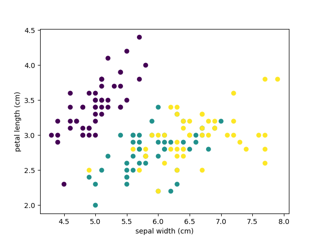
- 0과 3이면 a,b,c,d중 a,d선택
plt.scatter(iris.data[:,0], iris.data[:,3], c=iris.target)
plt.xlabel(iris.feature_names[1])
plt.ylabel(iris.feature_names[2])
plt.show()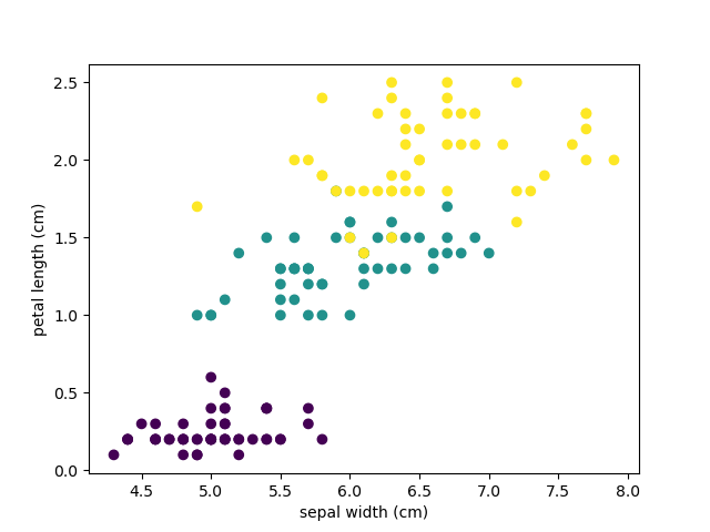
- 1과 2이면 a,b,c,d중 b,c선택
plt.scatter(iris.data[:,1], iris.data[:,2], c=iris.target)
plt.xlabel(iris.feature_names[1])
plt.ylabel(iris.feature_names[2])
plt.show()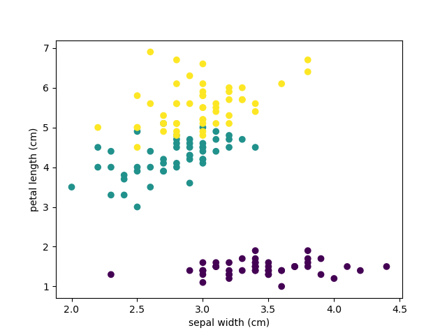
PCA실습
- new 데이터 생성
PCA의 계산과정을 필요없음 (함수에 내장됨)
n_components는 축소하고 싶은 dim을 나타냄
4차원의 데이터 -> 2차원의 데이터
from sklearn.decomposition import PCA
pca = PCA(n_components=2)
new_data = pca.fit_transform(iris.data)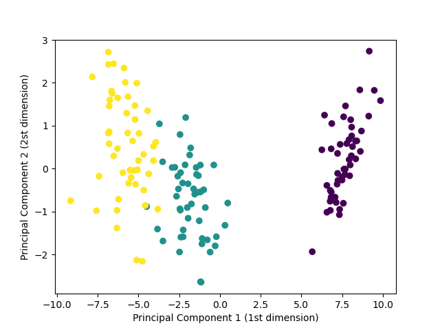
print(new_data)- PCA new 데이터 시각화
4차원의 데이터 -> 2차원의 데이터
plt.scatter(new_data[:,0], new_data[:,1], c=iris.target)
plt.xlabel("Principal Component 1 (1st dimension)")
plt.ylabel("Principal Component 2 (2st dimension)")
plt.show()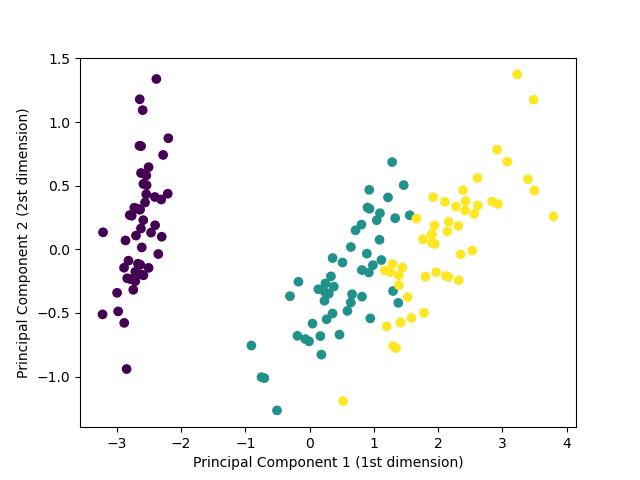
- PCA 3차원상에서의 시각화
pca = PCA(n_components=3)
new_data = pca.fit_transform(iris.data)
fig = plt.figure()
from mpl_toolkits import mplot3d
ax = plt.axes(projection='3d')
ax.scatter3D(new_data[:,0], new_data[:,1], new_data[:,2], c=iris.target)
plt.show()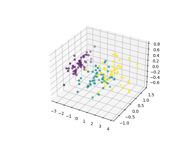
LDA실습
-
new 데이터 생성
4차원의 데이터를 2차원의 데이터로 줄인다.
from sklearn.discriminant_analysis import LinearDiscriminantAnalysis
iris = datasets.load_iris()
lda = LinearDiscriminantAnalysis(n_components=2)
new_data = lda.fit_transform(iris.data, iris.target) -
LDA new 데이터 시각화
4차원에서 -> 2차원의 데이터
plt.scatter(new_data[:,0], new_data[:,1], c=iris.target)
plt.xlabel("Principal Component 1 (1st dimension)")
plt.ylabel("Principal Component 2 (2st dimension)")
plt.show()