1. 최단 경로탐색
- 가장 짧은 경로를 찾는 알고리즘, '길 찾기'문제로 불린다.
- 그리디 알고리즘, DP 프로그래밍이 그대로 적용된다.
1) 다익스트라 최단 경로 알고리즘
- 가중치 그래프에서, 시작정점으로부터 다른 모드 정점까지의 최단 경로를 찾는 알고리즘
- 우선순위 큐를 사용
- 어렵게 생각하지 말자
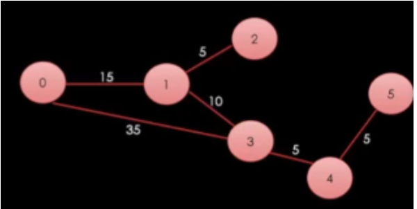
- 아래의 코드는 위의 그래프에서 각 노드로 가는 최소 비용을 출력해주는 코드다.
- 결국 경로를 들려가며 비용을 확인하면서 최단경로를 찾는 코드다
#include <iostream>
#include <vector>
#include <queue>
using namespace std;

struct Vertex
{
	// int data;
};

vector<Vertex> vertices;		// 정점 배열.
vector<vector<int>> adjacent;	// 정점간 연결 상태 저장 배열.

void CreateGraph()
{
	vertices.resize(6);	// 정점 6개 생성.

	// 정점간 연결 상태 저장.
	// adjacent[정점1][정점2] = adjacent[정점2][정점1] = 가중치 값.
	adjacent = vector<vector<int>>(6, vector<int>(6, -1));
	adjacent[0][1] = adjacent[1][0] = 15;
	adjacent[0][3] = adjacent[3][0] = 35;
	adjacent[1][2] = adjacent[2][1] = 5;
	adjacent[1][3] = adjacent[3][1] = 10;
	adjacent[3][4] = adjacent[4][3] = 5;
	adjacent[4][5] = adjacent[5][4] = 5;
}

// 정점과 가중치 값을 모아 놓은 구조체.
struct VertexCost
{
	// 구조체 생성자.
	VertexCost(int cost, int vertex) : cost(cost), vertex(vertex) { }

	// pq를 사용하기 위해 연산자 오버로딩 추가. (pq의 도장 깨기용)
	bool operator<(const VertexCost& other) const // const 필요.
	{
		return cost < other.cost;
	}

	// pq를 사용하기 위해 연산자 오버로딩 추가. (pq의 도장 깨기용)
	bool operator>(const VertexCost& other) const // const 필요.
	{
		return cost > other.cost;
	}

	int cost;
	int vertex;
};

void Dijkstra(int here)
{
	// 우선순위 큐를 최소힙으로 사용.
	priority_queue<VertexCost, vector<VertexCost>, greater<VertexCost>> pq;

	vector<int> best(6, INT32_MAX);	// 정점에 대한 최소 비용의 거리를 저장하는 배열.
	vector<int> parent(6, -1);		// 현재 정점을 발견한 이전의 정점을 저장하는 배열(정점 history 저장).

	pq.push(VertexCost(0, here));	// 시작 정점을 우선순위 큐에 저장
	best[here] = 0;					// 정점에 대한 최소 비용을 저장하는 배열.
	parent[here] = here;			// 특정 정점을 발견한 정점을 저장하는 배열. (정점 history 참고용)

	while (pq.empty() == false)
	{
		// 제일 좋은 후보를 찾는다.
		VertexCost v = pq.top();	// 우선순위 큐에서 제일 좋은 후보를 가져옴.
		pq.pop();

		here = v.vertex;			// 현재 정점 저장.
		int cost = v.cost;			// 현재 정점의 비용 저장.

		// 기존에 찾았던 비용보다 높은 경우 스킵.  (더 안좋은 경로를 찾은 경우)
		if (best[here] < cost)
			continue;

		// 방문
		cout << "방문!" << here << endl;

		for (int there = 0; there < 6; there++)
		{
			// 연결되지 않았으면 스킵
			if (adjacent[here][there] == -1)
				continue;

			// 다음 정점에 대한 현재 경로가 과거에 찾았던 경로보다 안좋으면 스킵.
			int nextCost = best[here] + adjacent[here][there]; // 현재 정점부터 다음 정점까지 비용 + 이전 정점부터 현재 정점까지 비용.
			if (nextCost >= best[there])
				continue;

			// 지금까지 찾은 경로 중 최단 경로의 정점임. = 갱신
			// 나중에 더 좋은 경로를 찾으면 언제든 갱신될 수 있음.
			best[there] = nextCost;
			parent[there] = here;
			pq.push(VertexCost(nextCost, there));
		}
	}

    // 경로 history와 각 정점에 대한 최소 비용 출력.
	cout << endl;
	cout << "경로 history" << endl;
	for (int i = 0; i < parent.size(); i++)
	{
		cout << "현재 정점 : " << i << ", 이전 정점 : " << parent[i] << endl;
	}
	cout << endl;

	cout << "비용" << endl;
	for (int i = 0; i < best.size(); i++)
	{
		cout << "정점 : " << i << ", 비용 : " << best[i] << endl;
	}
}

int main()
{
	CreateGraph();

	Dijkstra(0);
}
2. 벨만포드 알고리즘
- 한노드에서 목표노드로 가는데 걸리는 최소비용, 다익스트라와 동일한 점
- 다익스트라에선 간선이 음수일 때 최단경로를 구할 수 없다.
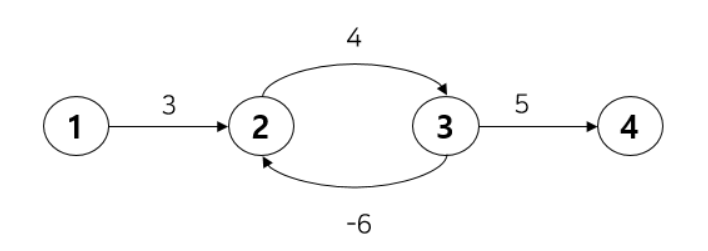
- 위 사진의 경우 다익스트라로 탐색할경우 무한히 작아진다.
- 이점을 보완한 것이 벨만포드, but 시간복잡도가 좀 더 높다.
- 다익스트라가 노드를 지나면서 최단거리를 구한다면 벨만포드는 해당 노드의 모든 간선에 대해 거리를 업데이트하며 최단거리를 구한다.
#include <iostream>
#include <vector>
#include <limits>

using namespace std;

struct Edge {
    int src, dest, weight;
};

class BellmanFord {
private:
    int V, E;
    vector<Edge> edges;
public:
    BellmanFord(int V, int E) : V(V), E(E) {
        edges.resize(E);
    }

    void addEdge(int idx, int u, int v, int w) {
        edges[idx].src = u;
        edges[idx].dest = v;
        edges[idx].weight = w;
    }

    void shortestPath(int src) {
        vector<int> dist(V, numeric_limits<int>::max());
        dist[src] = 0;

        for (int i = 0; i < V - 1; i++) {
            for (int j = 0; j < E; j++) {
                int u = edges[j].src;
                int v = edges[j].dest;
                int weight = edges[j].weight;

                if (dist[u] != numeric_limits<int>::max() && dist[u] + weight < dist[v]) {
                    dist[v] = dist[u] + weight;
                }
            }
        }

        for (int j = 0; j < E; j++) {
            int u = edges[j].src;
            int v = edges[j].dest;
            int weight = edges[j].weight;

            if (dist[u] != numeric_limits<int>::max() && dist[u] + weight < dist[v]) {
                cout << "The graph contains a negative-weight cycle" << endl;
                return;
            }
        }

        for (int i = 0; i < V; i++) {
            cout << "Vertex " << i << " distance from source: " << dist[i] << endl;
        }
    }
};

int main() {
    int V = 5, E = 8;
    BellmanFord graph(V, E);

    graph.addEdge(0, 0, 1, -1);
    graph.addEdge(1, 0, 2, 4);
    graph.addEdge(2, 1, 2, 3);
    graph.addEdge(3, 1, 3, 2);
    graph.addEdge(4, 1, 4, 2);
    graph.addEdge(5, 3, 2, 5);
    graph.addEdge(6, 3, 1, 1);
    graph.addEdge(7, 4, 3, -3);

    graph.shortestPath(0);

    return 0;
}
3. 이제부터 슬슬 어렵다.
벨만포드 알고리즘 링크에 두번째꺼는 그림과 표의 설명이 잘못 되었다. 놀라지 말시길
Reference
- 다익스트라 최단경로 알고리즘
https://velog.io/@taeil314/AlgorithmC-%EB%8B%A4%EC%9D%B5%EC%8A%A4%ED%8A%B8%EB%9D%BC-%EC%B5%9C%EB%8B%A8-%EA%B2%BD%EB%A1%9C-%EC%95%8C%EA%B3%A0%EB%A6%AC%EC%A6%98-Dijkstra - 벨만포드 알고리즘
https://yabmoons.tistory.com/365
https://roytravel.tistory.com/340#:~:text=%EB%8B%A4%EC%9D%B5%EC%8A%A4%ED%8A%B8%EB%9D%BC%EB%8A%94%20%EC%B6%9C%EB%B0%9C%20%EB%85%B8%EB%93%9C,%EC%9D%98%20%EC%B5%9C%EC%86%8C%20%EB%B9%84%EC%9A%A9%EC%9D%84%20%EA%B5%AC%ED%95%9C%EB%8B%A4.

좋은 지식 나누어요