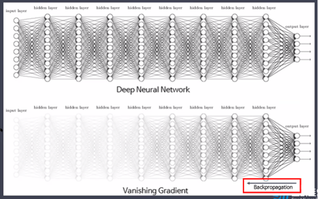
오차 역전파(Back Propagation)
-
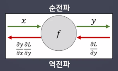
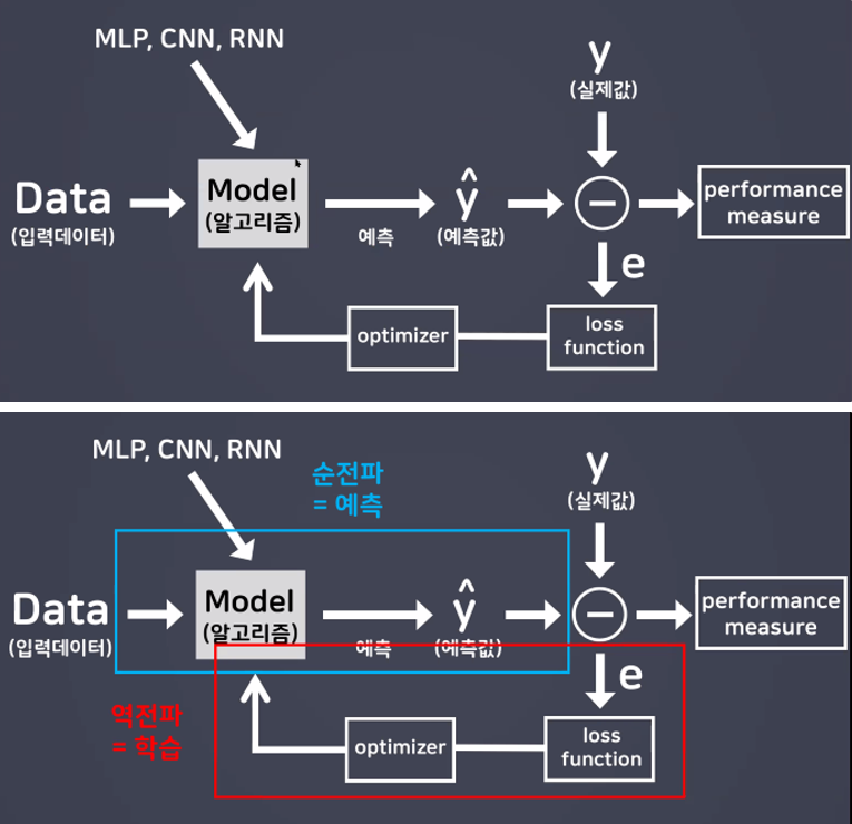
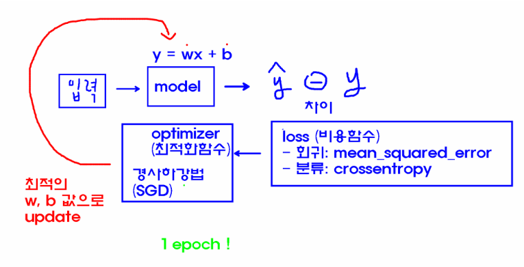
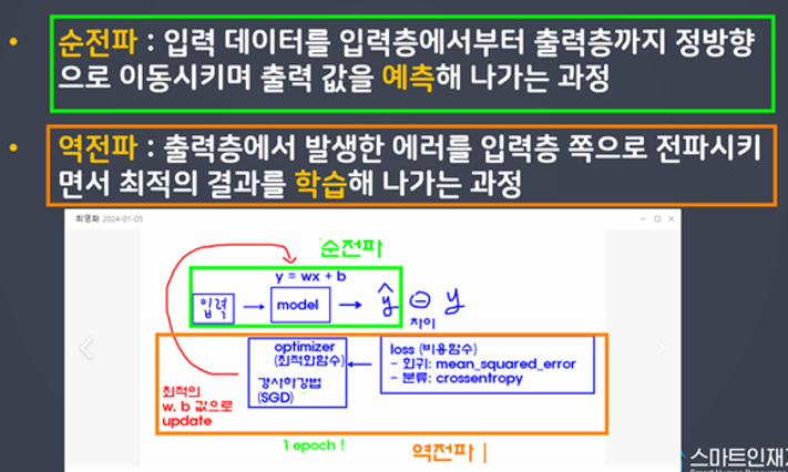
순전파
입력데이터를 입력층에서부터 출력층까지 정방향으로 이동시키며 출력 값을 예측해 나가는 과정 -
역전파
출력층에서 발생한 에러를 입력층 쪽으로 전파시키면서 최적의 결과를 학습해 나가는 과정
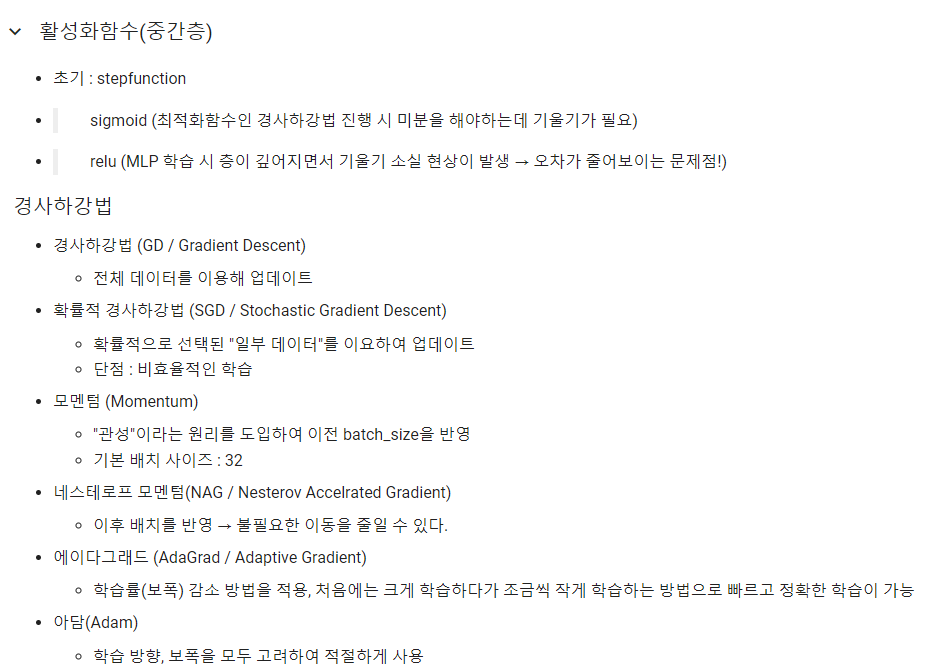
- Sigmoid 함수의 문제점
기울기 소실 문제(Vanishing Gradient)
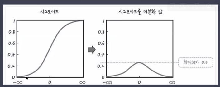 → 최대치가 0.3이 아니라 0.2
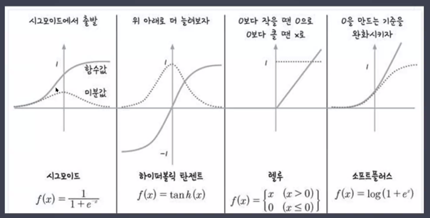
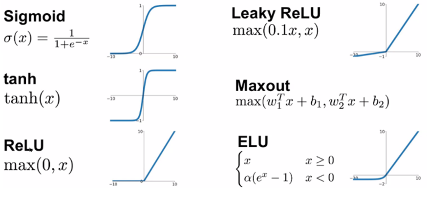
- 활성화 함수(Activation)의 종류
- 최적화 함수(optimizer)의 종류
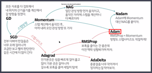
경사하강법(Gradient Descent Algorithm)
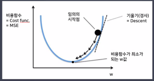
- 경사하강법(Gradient Descent)

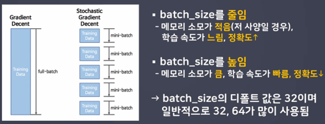
- 확률적경사하강법(Stochasitc Gradient Descent)
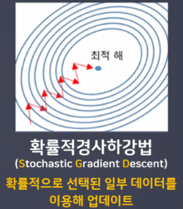
- 확률적경사하강법 장단점
- 배치 GD보다 더 빨리, 더 자주 업데이트를 한다.
- 지역 최저점을 빠져 나갈 수 있다.
- 탐색 경로가 비효율적이다. 하지만 결과는 잘 나오는 편!(진폭이 크고 불안정)
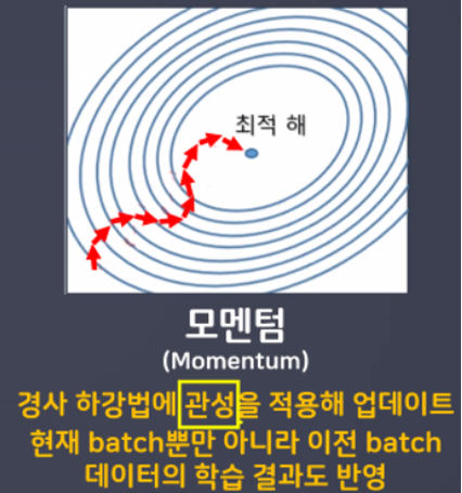
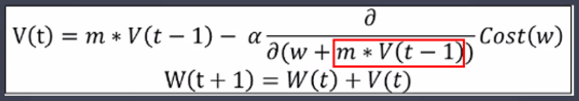
- 모멘텀
- 네스테로프 모멘텀(Nesterov Accelrated Gradient)
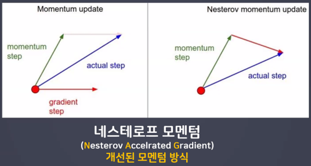
- 네스테로프 모멘텀 특징
- w, b값 업데이트 시 모멘텀 방식으로 먼저 더한 다음 계산
- 미리 해당 방향으로 이동한다고 가정하고 기울기를 계산해본 뒤 실제 업데이트 반영
- 불필요한 이동을 줄일 수 있다.
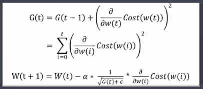
- 에이다그래드(Adaptive Gradient)
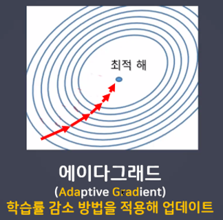
- 에이다그래드 특징
- 학습을 진행하면서 학습률을 점차 줄여가는 방법
- 처음에는 크게 학습하다가 조금씩 작게 학습한다.
- 학습을 빠르고 정확하게 할 수 있다.
- Batch_size
일반적으로 PC메모리의 한계 및 속도 저하 때문에 대부분의 경우에는 한번의 epoch에 모든 데이터를 한꺼번에 집어넣기가 힘듦

실습
- 라이브러리 불러오기
import numpy as np
import pandas as pd
import matplotlib.pyplot as plt
from tensorflow.keras import Sequential
from tensorflow.keras.layers import Dense, InputLayer, Flatten- optimizer 불러오기(최적화함수 클래스 불러와서 사용해보자!)
from tensorflow.keras.optimizers import SGD, Adam- 데이터 불러오기(4개의 변수에 담기! X_train, y_train, X_test, y_test)
from tensorflow.keras.datasets import mnist
(X_train, y_train), (X_test, y_test) = mnist.load_data()- 데이터 확인
X_train.shape, y_train.shape, X_test.shape, y_test.shape
- model1 / h1
# 1. 모델 설계(model1, model2, model3)
# 뼈대
model1 = Sequential()

#입력층
model1.add(InputLayer(input_shape = (28, 28)))

# 중간층(총 5개의 층, units = 64, 128, 256, 128, 64)
model1.add(Flatten())
model1.add(Dense(units = 64, activation = 'sigmoid'))
model1.add(Dense(units = 128, activation = 'sigmoid'))
model1.add(Dense(units = 256, activation = 'sigmoid')) # 항아리 모양처럼 쌓아주자
model1.add(Dense(units = 128, activation = 'sigmoid'))
model1.add(Dense(units = 64, activation = 'sigmoid'))

# 출력층
model1.add(Dense(units = 10, activation = 'softmax'))

# 2. 학습 방법 및 평가 방법 설정 # optimizer : 'SGD'
model1.compile(loss = 'sparse_categorical_crossentropy',
               optimizer = 'SGD',
               metrics = ['accuracy'])

# 3. 학습(h1, h2, h3)
h1 = model1.fit(X_train, y_train,
                validation_split = 0.2,
                epochs = 20)
# 4. 평가
model1.evaluate(X_test, y_test)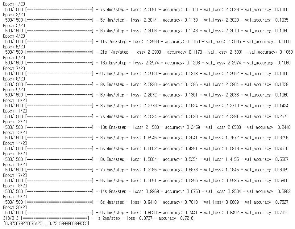
- model2 / h2
# 1. 모델 설계(model1, model2, model3)
# 뼈대
model2 = Sequential()

# 입력층
model2.add(InputLayer(input_shape = (28, 28)))

# 중간층(총 5개의 층, units = 64, 128, 256, 128, 64)
model2.add(Flatten())

model2.add(Dense(units = 64, activation = 'relu'))
model2.add(Dense(units = 128, activation = 'relu'))
model2.add(Dense(units = 256, activation = 'relu'))
model2.add(Dense(units = 128, activation = 'relu'))
model2.add(Dense(units = 64, activation = 'relu'))

#출력층
model2.add(Dense(units = 10, activation = 'softmax'))

# 2. 학습 방법 및 평가 방법 설정 # optimizer : 'SGD'
model2.compile(loss = 'sparse_categorical_crossentropy',
               optimizer = 'SGD',
               metrics = ['accuracy'])

# 3. 학습(h1, h2, h3)
h2 = model2.fit(X_train, y_train,
                validation_split = 0.2,
                epochs = 20)
# 4. 평가
model2.evaluate(X_test, y_test)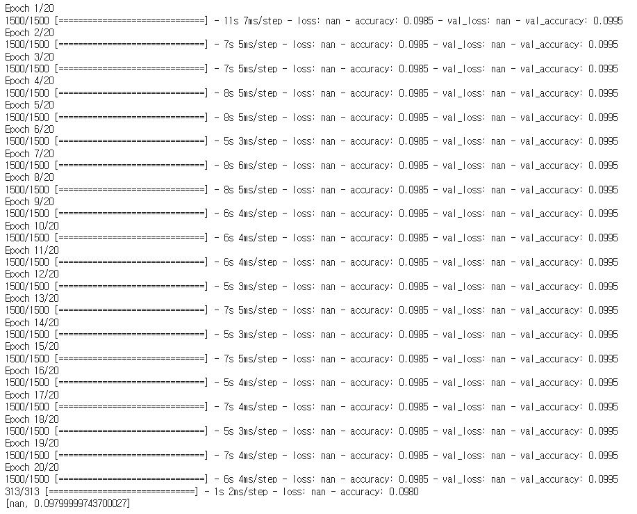
- model2 / h2 낮춰서 사용해보기
# 1. 모델 설계(model1, model2, model3)
# 뼈대
model2 = Sequential()

# 입력층
model2.add(InputLayer(input_shape = (28, 28)))

# 중간층(총 5개의 층, units = 64, 128, 256, 128, 64)
model2.add(Flatten())

model2.add(Dense(units = 64, activation = 'relu'))
model2.add(Dense(units = 128, activation = 'relu'))
model2.add(Dense(units = 256, activation = 'relu'))
model2.add(Dense(units = 128, activation = 'relu'))
model2.add(Dense(units = 64, activation = 'relu'))

#출력층
model2.add(Dense(units = 10, activation = 'softmax'))

# 2. 학습 방법 및 평가 방법 설정 # optimizer : 'SGD'
model2.compile(loss = 'sparse_categorical_crossentropy',
               optimizer = SGD(learning_rate=0.001),
               # SGD 함수의 기본 학습률 0.01 → 0.001(학습률 낮춰보기)
               # 중간층의 활성화함수를 relu로 변경하면서 오차가 줄어들지 않게됨
               # 에러가 큰 값이 그대로 전달되는 것을 줄여주기 위함
               metrics = ['accuracy'])

# 3. 학습(h1, h2, h3)
h2 = model2.fit(X_train, y_train,
                validation_split = 0.2,
                epochs = 20)
# 4. 평가
model2.evaluate(X_test, y_test)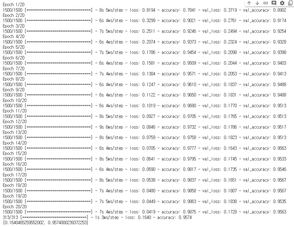
- model3 / h3
# 1. 모델 설계(model1, model2, model3)
# 뼈대
model3 = Sequential()

# 입력층
model3.add(InputLayer(input_shape = (28, 28)))

# 중간층(총 5개의 층, units = 64, 128, 256, 128, 64)
model3.add(Flatten())

model3.add(Dense(units = 64, activation = 'relu'))
model3.add(Dense(units = 128, activation = 'relu'))
model3.add(Dense(units = 256, activation = 'relu'))
model3.add(Dense(units = 128, activation = 'relu'))
model3.add(Dense(units = 64, activation = 'relu'))

# 출력층
model3.add(Dense(units = 10, activation = 'softmax'))

# 2. 학습 방법 및 평가 방법 설정 # optimizer : 'Adam'
model3.compile(loss = 'sparse_categorical_crossentropy',
               optimizer = 'Adam',
               metrics = ['accuracy'])

# 3. 학습(h1, h2, h3)
h3 = model3.fit(X_train, y_train,
                validation_split = 0.2,
                epochs = 20)

# 4. 평가
model3.evaluate(X_test, y_test)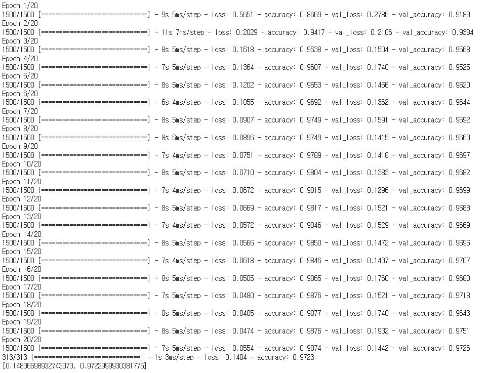
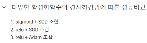
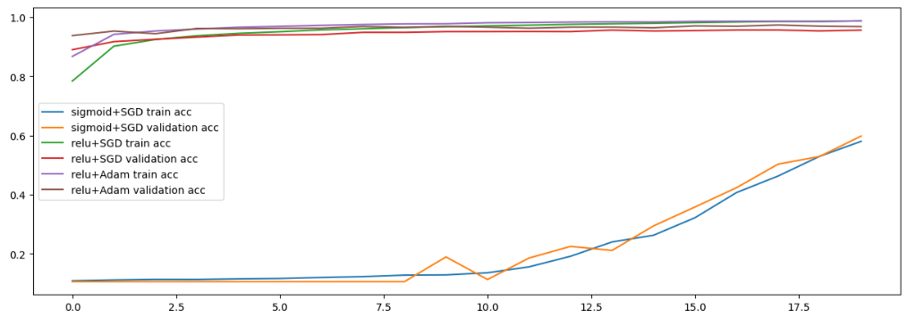
- 시각화(3개 모델 한 번에 시각화 / 총 6개의 직선 비교)
# h1 → accuracy, val_accuracy
# h2 → accuracy, val_accuracy
# h3 → accuracy, val_accuracyplt.figure(figsize = (15,5))
plt.plot(h1.history['accuracy'], label = 'sigmoid+SGD train acc')
plt.plot(h1.history['val_accuracy'], label = 'sigmoid+SGD validation acc')
plt.plot(h2.history['accuracy'], label = 'relu+SGD train acc')
plt.plot(h2.history['val_accuracy'], label = 'relu+SGD validation acc')
plt.plot(h3.history['accuracy'], label = 'relu+Adam train acc')
plt.plot(h3.history['val_accuracy'], label = 'relu+Adam validation acc')
plt.legend() # 범례
plt.show()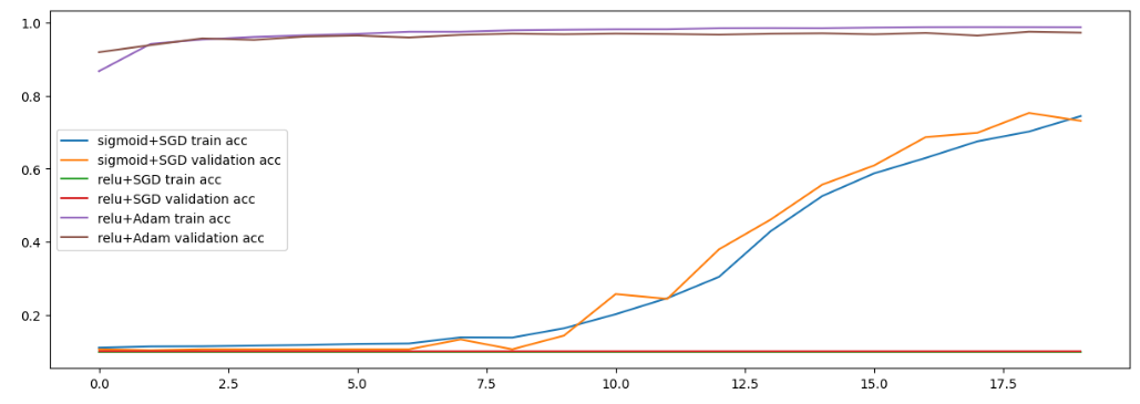
- 낮췄을 때
콜백함수
from tensorflow.keras.callbacks import ModelCheckpoint, EarlyStopping
# 모델 중간 저장 : ModelCheckpoint
# 모델 중간 멈춤 : EarlyStopping- 모델 저장 객체 생성
# 모델을 저장 할 경로 설정(경로 변경 후 사용 할 것)
model_path = '/content/drive/MyDrive/Colab Notebooks/DeepLearning/data/digit_model/dm_{epoch:02d}_{val_accuracy:0.2f}.hdf5'

mc = ModelCheckpoint(filepath = model_path, # 모델을 저장 할 경로
                     verbose = 1,
                     # 로그출력 : 0(로그출력 X), 1(로그출력 O), 몇 번째에 저장되는지 확인이 가능
                     save_best_only = True,
                     # 모델 성능이 최고점을 갱신할 때만 저장(False 설정 시 매 epoch 마다 저장)
                     monitor = 'val_accuracy') # 모델의 성능을 확인 할 기준
                     # 일반화 확인을 위하여 val_accuracy로 선택!

# 모델 저장 객체 생성 완료~
# 하지만 사용은 아직 안한 것! → 학습 시 객체를 불러와서 사용 할 것!- 조기 학습 중단
es = EarlyStopping(monitor='val_accuracy', # 학습을 중단 할 기준
                   verbose = 1, # 로그출력
                   patience = 10) # 모델 성능 개선을 기다리는 최대 횟수

# 조기 학습 중단 객체 생성 완료~- 모델 설계 ~ 평가
# 1. 모델 설계
# 뼈대
model1 = Sequential()

#입력층
model1.add(InputLayer(input_shape = (28, 28)))

# 중간층(총 5개의 층, units = 64, 128, 256, 128, 64)
model1.add(Flatten())
model1.add(Dense(units = 64, activation = 'sigmoid'))
model1.add(Dense(units = 128, activation = 'sigmoid'))
model1.add(Dense(units = 256, activation = 'sigmoid')) # 항아리 모양처럼 쌓아주자
model1.add(Dense(units = 128, activation = 'sigmoid'))
model1.add(Dense(units = 64, activation = 'sigmoid'))

# 출력층
model1.add(Dense(units = 10, activation = 'softmax'))

# 2. 학습 방법 및 평가 방법 설정
model1.compile(loss = 'sparse_categorical_crossentropy',
               optimizer = 'SGD',
               metrics = ['accuracy'])

# 3. 학습
h1 = model1.fit(X_train, y_train,
                validation_split = 0.2,
                epochs = 1000,
                callbacks = [mc, es])
# 4. 평가
model1.evaluate(X_test, y_test)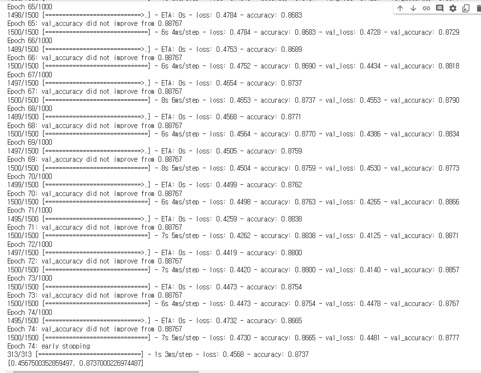
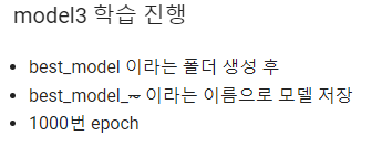
- 모델 저장 객체 생성
# 모델을 저장 할 경로 설정(경로 변경 후 사용 할 것)
model_path = '/content/drive/MyDrive/Colab Notebooks/DeepLearning/data/best_model/dm_{epoch:02d}_{val_accuracy:0.2f}.hdf5'

mc1 = ModelCheckpoint(filepath = model_path, # 모델을 저장 할 경로
                     verbose = 1,
                     # 로그출력 : 0(로그출력 X), 1(로그출력 O), 몇 번째에 저장되는지 확인이 가능
                     save_best_only = True,
                     # 모델 성능이 최고점을 갱신할 때만 저장(False 설정 시 매 epoch 마다 저장)
                     monitor = 'val_accuracy') # 모델의 성능을 확인 할 기준
                     # 일반화 확인을 위하여 val_accuracy로 선택!

# 모델 저장 객체 생성 완료~
# 하지만 사용은 아직 안한 것! → 학습 시 객체를 불러와서 사용 할 것!- 조기 학습 중단
es1 = EarlyStopping(monitor='val_accuracy', # 학습을 중단 할 기준
                   verbose = 1, # 로그출력
                   patience = 10) # 모델 성능 개선을 기다리는 최대 횟수

# 조기 학습 중단 객체 생성 완료~- 모델 설계 ~ 평가
# 1. 모델 설계(model1, model2, model3)
# 뼈대
model3 = Sequential()

# 입력층
model3.add(InputLayer(input_shape = (28, 28)))

# 중간층(총 5개의 층, units = 64, 128, 256, 128, 64)
model3.add(Flatten())

model3.add(Dense(units = 64, activation = 'relu'))
model3.add(Dense(units = 128, activation = 'relu'))
model3.add(Dense(units = 256, activation = 'relu'))
model3.add(Dense(units = 128, activation = 'relu'))
model3.add(Dense(units = 64, activation = 'relu'))

# 출력층
model3.add(Dense(units = 10, activation = 'softmax'))

# 2. 학습 방법 및 평가 방법 설정 # optimizer : 'Adam'
model3.compile(loss = 'sparse_categorical_crossentropy',
               optimizer = 'Adam',
               metrics = ['accuracy'])

# 3. 학습(h1, h2, h3)
h3 = model3.fit(X_train, y_train,
                validation_split = 0.2,
                epochs = 1000, batch_size = 128,
                callbacks = [mc1, es1])

# 4. 평가
model3.evaluate(X_test, y_test)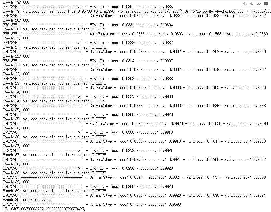
직접 만든 손글씨 데이터

- 직접 작성한 손글씨 → 이미지 데이터
# 파이썬에서 이미지를 처리하는 라이브러리
import PIL.Image as pimg- 이미지 불러오기
img = pimg.open('/content/drive/MyDrive/Colab Notebooks/DeepLearning/data/손글씨/0.png')
plt.imshow(img, cmap = 'gray')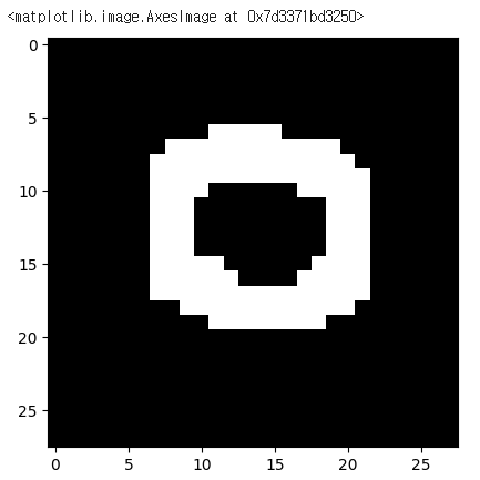
- 전처리
# 이미지 컬러이미지 → 흑백 이미지로 변경
img = img.convert('L')- 이미지 데이터를 배열로 변환
img = np.array(img)
img.shape
- 원본 이미지에 했던 전처리를 그대로 해주어야 한다.
# 2차원 → 1차원(flatten)
testimg = img.reshape(1, 28, 28, 1)
testimg = testimg.astype('float32')/255
testimg.shape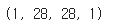
- 우리의 best_model 불러와서 확인하기
from tensorflow.keras.models import load_model
best_model = load_model('/content/drive/MyDrive/Colab Notebooks/DeepLearning/data/best_model/dm_19_0.97.hdf5')- 평가
best_model.evaluate(X_test, y_test)
- 우리의 손글씨 넣어서 예측하기
best_model.predict(testimg)
# 10개의 확률값 출력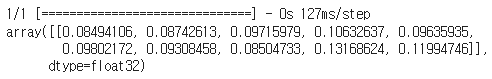
- 하나의 클래스를 출력하고 싶다면? (argmax)
best_model.predict(testimg).argmax()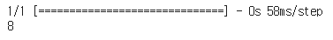
- 최종정리
# test 데이터에 대해서는 높은 성능을 보였으나
# 우리가 작성한 손글씨에서는 낮은 정확도를 보이더라
# 왜?
# 제공된 데이터는 데이터의 크기와 모양이 일정하게 정제되어있음
# 하지만 우리의 데이터는 모양과 위치가 학습 데이터와 일치하지 않기 떄문에 결과가 별로

# Dense 층은 1차원 데이터만 학습이 가능하더라
# 이미지는 2차원 데이터(우리가 억지로 1차원으로 만들어서 학습)
# 픽셀 하나하나의 색 정보만 학습할뿐 이미지 전체적인 특성을 학습하는 것이 아니다보니
# 숫자의 모양, 크기, 위치가 변경되면 예측률이 떨어지더라~
노는게 제일 좋아~!