Statistical Inference about Two Populations

두 모집단을 비교해보자

Difference in two means with known population variances

use z statistic

두 모평균의 차이는 $\bar x_1-\bar x_2$로 나타낼 수 있다.
이를 예시에 적용해보면, 두 브랜드의 치약이 동일하게 효과적인가? / 두 브랜드의 타이어가 다르게 닳는가? 등이 있다.
CLT에 따라, x_1과 x_2의 표본의 크기가 모두 충분히 클 때($\geq 30$), $\bar x_1-\bar x_2$도 정규분포를 따른다.

$\bar x_1-\bar x_2$의 평균(기댓값)은 $\mu_1-\mu_2$, 분산은 $\frac{\sigma_1^2}{n_1}+\frac{\sigma_2^2}{n_2}$이다.

그러면 Z값으로 표준화시켜보자.

이 값을 검정하는 데에도 활용할 수 있다.

ex. Suppose we want to conduct a hypothesis test to determine whether the average annual wage for an auditing manager is different from the average annual wage of an advertising manager, where auditing managers are population 1 and advertising managers are population 2.

• A random sample of 34 auditing managers is taken.
• A similar random sample is taken of 32 advertising managers.
• The sample of auditing managers has a sample mean of $98,959 and a known population standard deviation of $12,709
• The sample of advertising managers has a sample mean of $95,433 and a known population standard deviation of $15,997
• Let α = 0.05, giving a z value of 1.96

H0의 값을 넣어서 계산해본다.

-> Since 0.99 < 1.96, we fail to reject the null hypothesis
1.96보다 작은 값이 나왔다. 즉 기각역에 포함이 되지 않으므로 H0은 유의수준 0.05 하에서 기각되지 않는다.

Confidence Interval

모평균 추정에서의 신뢰구간은 다음과 같았다. $\bar{x}-z_{\alpha / 2} \frac{\sigma}{\sqrt{n}} \leq \mu \leq \bar{x}+z_{\alpha / 2} \frac{\sigma}{\sqrt{n}}$
평균 + z값*표준편차다.

두 모평균의 추정도 상응하는 값을 넣으면 신뢰구간을 구할 수 있다.

Difference in two means with unknown population variances

use t statistic

samples are independent라는 가정이 필요하다.
해당 경우에서 우리는 모분산을 모르기 때문에, 두 모집단의 분산이 같은 경우(등분산성)와 다른 경우로 나누어 생각해보아야 한다.

1) 등분산 가정 $\sigma_1^2=\sigma_2^2=\sigma^2$

두 모집단의 분산이 같을 경우, 식을 다음과 같이 정리할 수 있다.

그러면 우리는 추정해야 하는 모분산이 공통 모분산 $\sigma^2$으로 하나가 된다.
공통 모분산 $\sigma^2$의 추정량은 $S^2_p$이고, 그 추정값은 다음과 같다. 이렇게 계산된 표본분산은 합동표본분산(pooled sample variance)라고 한다.

Note that $\mathbb{E}\left[s_p^2\right]=\sigma^2$
Proof: $\mathbb{E}\left[s_p^2\right]=\frac{\left(n_1-1\right) \mathbb{E}\left[s_1^2\right]+\left(n_2-1\right) \mathbb{E}\left[s_2^2\right]}{n_1+n_2-2}=\frac{\left(n_1-1\right) \sigma^2+\left(n_2-1\right) \sigma^2}{n_1+n_2-2}=\sigma^2$

모집단의 분포가 독립이고 등분산 정규분포를 하는 경우 $\bar x_1 - \bar x_2$의 검정통계량인

은 자유도가 n1+n2-2인 t분포를 따르게 된다.

2) 이분산 가정

두 모집단의 분산이 다르다고 가정하는 경우이다. 이 경우 s1과 s2를 구분해야 하기 때문에 다음과 같은 t값과 자유도의 공식이 나온다. 이 공식은 unpooled formula로 알려져 있다.

자유도의 소수점 이하는 버리고 정수부분만 사용한다.

(참고) 강의안에는 안 나왔는데, 신뢰구간은 다음과 같다.

Difference in two dependent populations

use t statistic

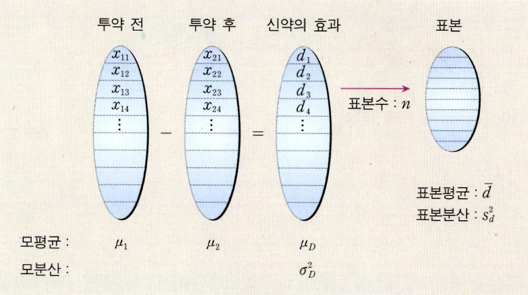
독립이 아닌 두 모집단의 차이이다. dependent samples, related samples를 다루기 위한 수단이다. Matched-pairs, correlated t test 로도 불린다.
예를 들면, 다이어트하기 전과 한 달 후의 몸무게처럼 동일한 개체에 대해 실험 전과 실험 후의 측정값의 차이를 추론할 수 있다.
두 모집단의 표본의 크기는 같아야 한다.

$\bar{d}=\frac{1}{n} \sum_{i=1}^n d_i$: 차이의 평균이다.
$s_d=\sqrt{\frac{\sum_{i=1}^n\left(d_i-\bar{d}\right)^2}{n-1}}$: 차이의 표준편차다.
n: 짝의 개수
d_i: ith 짝의 차이
D: 모집단의 차이($\mu_D$)

---

예시

---

이렇게 데이터가 주어졌을 경우 각 짝 자료에 대해 차이(d)를 구하고, 그 평균과 분산도 직접 계산한다.

$n=9, \bar{d}=-5.033, s_d=21.599$

귀무가설을 두 모집단에 차이가 없다는 것으로 설정했기 때문에 D=0 이다.

−3.355 < − 0.70 < 3.355 이기 때문에 H0 기각 실패

---

신뢰구간은 다음과 같다.

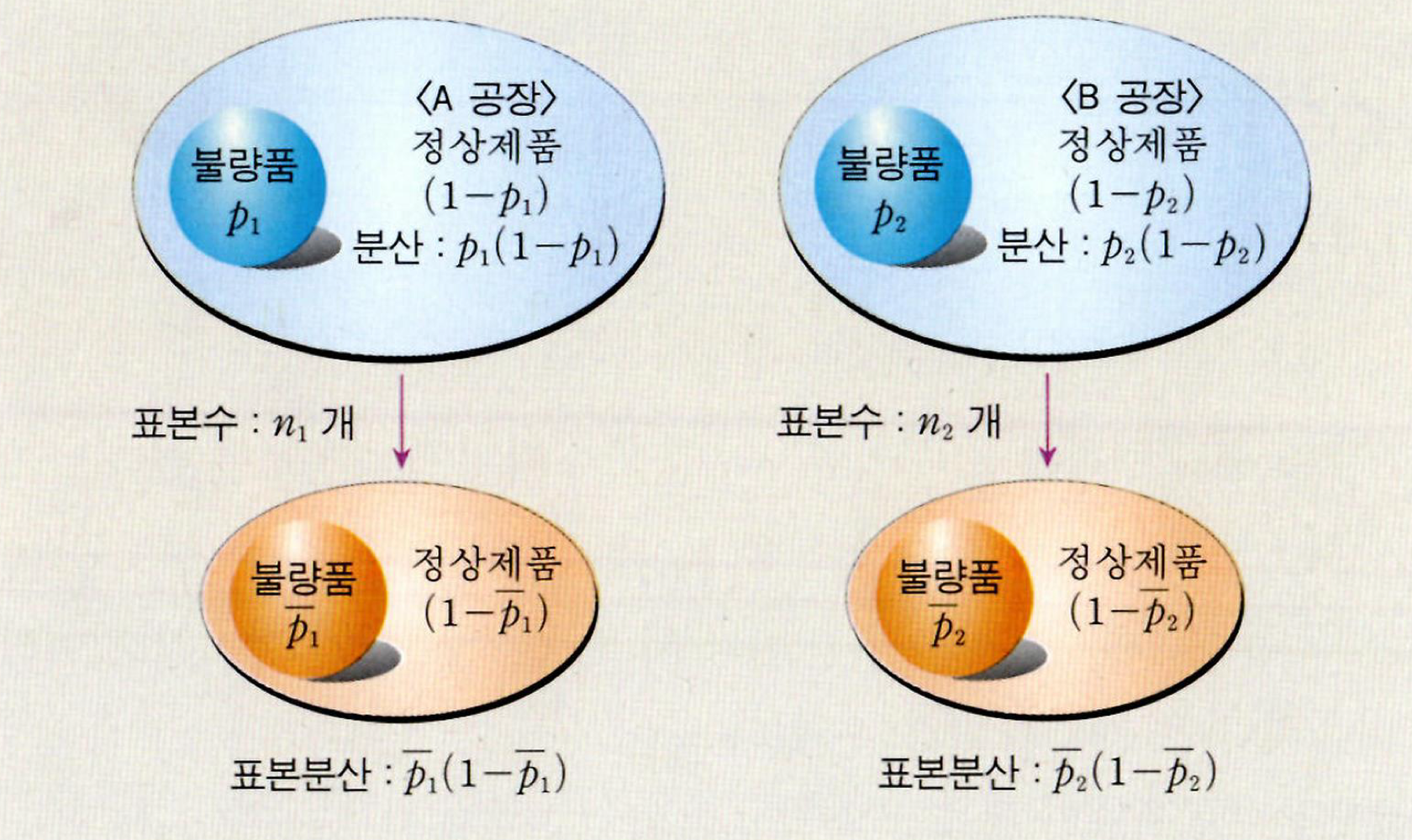
Difference in two population proportions

use z statistic

A집단의 불량률이 높은지, B집단의 불량률이 높은지 검정할 수 있다.

$p_1, p_2$는 모비율이다.
$q_1=1-p_1, q_2=1-p_2$

CLT를 적용하려면, $n_1 \hat{p}_1, n_1 \hat{q}_1, n_2 \hat{p}_2, n_2 \hat{q}_2>5$여야 함을 잊지 말아야 한다.

다른 검정통계량과 마찬가지로 평균과 표준편차를 활용해 계산한다.

이때 p1과 p2의 값을 추정해야 한다.

$\bar{p}$ 값은 다음과 같이 추정할 수 있다.

Difference in two population variances

use F distribution

F분포란?

카이제곱분포는 한 정규모집단의 모분산을 추론하는 데에 사용되었다면, F분포는 두 정규모집단의 분산을 비교하는 데에 사용된다.

독립적인 카이제곱 변수 $\chi_n^2$와 $\chi_m^2$이 있을 때, $X=\frac{\chi_n^2 / n}{\chi_m^2 / m}$는 자유도가 n, m인 F분포를 따른다.

• If $X \sim t_n$ then $X^2 \sim F_{1, n}$
• $F_{\alpha, n, m}$ is defined to be the value that satisfies $\operatorname{Pr}\left(X>F_{\alpha, n, m}\right)=\alpha$ where $\operatorname{Pr}\left(X>F_{\alpha, n, m}\right)=\alpha$
• $F_{1-\alpha, m, n}=\frac{1}{F_{\alpha, n, m}}$
  • $P\left(X>F_{a, n, m}\right)=a$
  • $P\left(1 / X<1 / F_{a, n, m}\right)=a$
  • $P\left(1 / X>1 / F_{a, n, m}\right)=1-a$
• $1 / X=Y \sim F_{m, n}$
  • Thus $F_{1-a, m, n}=1 / F_{a, n, m}$

검정

• samples must be random and independent
• Each population must have a normal distribution

$H_0: \sigma_1^2=\sigma_2^2$
test statistic: $F=\frac{s_1^2}{s_2^2} \sim F_{n_1-1, n_2-1}$

step1.

(two-tailed)

step2.
Since the population is normally distributed, the F test for the ratio of the variances can be used

step3.
type I-error : $\alpha=0.05$

step4.
Two-tailed test with $\alpha / 2=0.025, \nu_1=n_1-1=9, \nu_2=n_2-1=11$
The critical F value for the upper tail is $F_{0.025,9,11} = 3.59$

• How to compute the lower tail value using the table?
  • Use $1 / F_{0.025,11,9} \approx 1 / 3.92=0.26$. Why?
  • Remember the property: $F_{1-\alpha, m, n}=\frac{1}{F_{\alpha, n, m}}$

step5.
데이터에서 표본분산 구했다고 가정
$F=\frac{s_1^2}{s_2^2}=\frac{0.11378}{0.02023}=5.62$

The observed F value 5.62 is greater than the upper-tail critical value 3.59. Thus, reject the null hypothesis and conclude that the population variances are not equal.