Quantitative Trading with Python and Pandas #1 - Strategy

When I was started learning about quantitative trading, I was looking for the simplest algorithm with a good enough strategy that guarantees good return with backtesting.

And, I implemented two simple strategies.

1. Buying at a Golden Cross, and Selling at a Death Cross using a Simple Moving Average.

2. Buy even more if Adaptive Moving Average trends higher.

Steps :

I imported the data using a quandl API rather than saving into my SQL.

import quandl
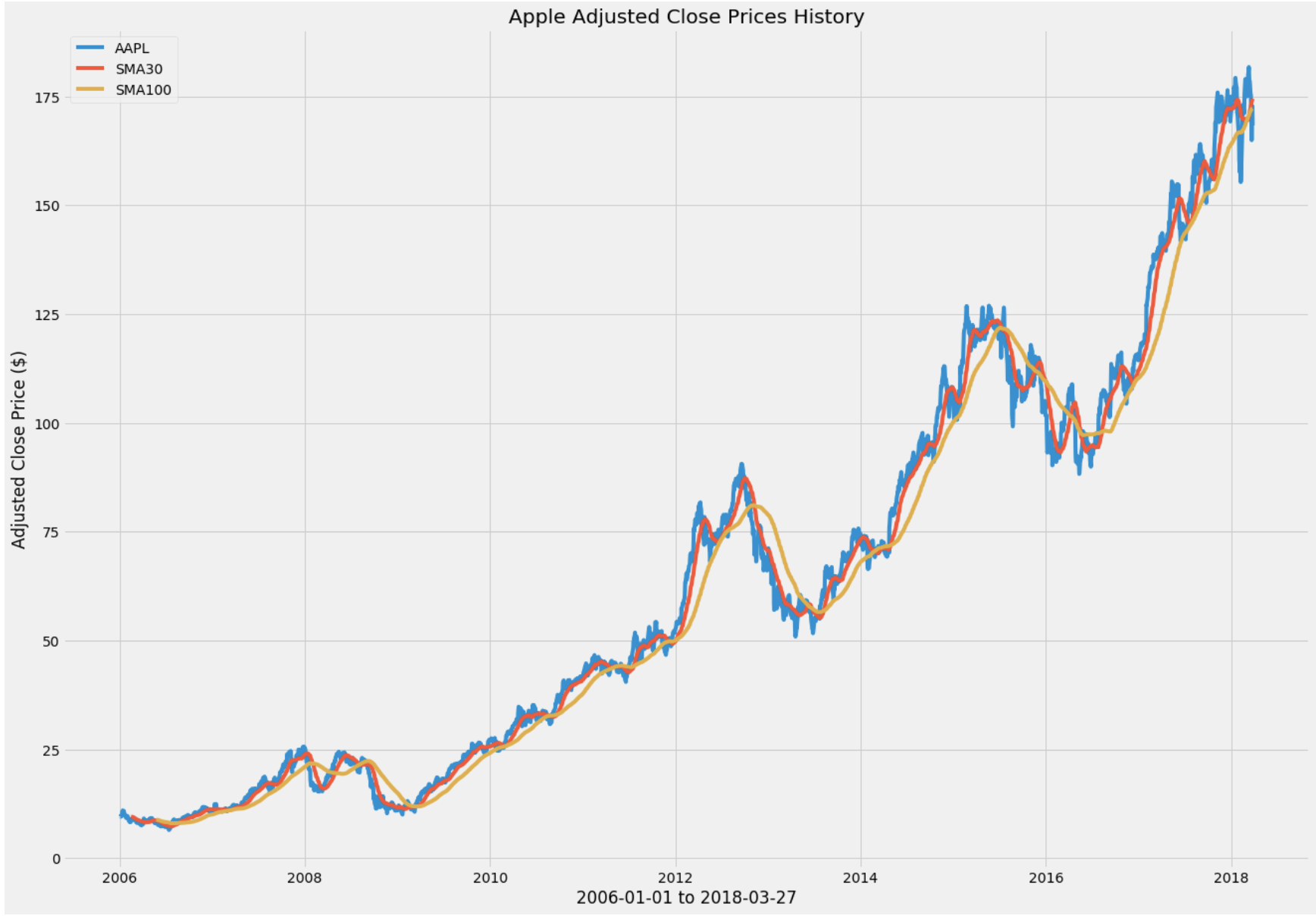
data = quandl.get("WIKI/AAPL", start_date="2006-01-01", end_date="2020-10-30")

Then, I caculated a simple moving aveage with the window of 30days and 100 days. Historically speaking, calculating SMA with 50 days and 200 days is the most conventional way, but I went with 30 and 100 days as I believed the window of 2006 to 2020 wasn't enough of a data.

SMA30 = pd.DataFrame()
SMA30['Adj. Close'] = data['Adj. Close'].rolling(window=30).mean()

SMA100 = pd.DataFrame()
SMA100['Adj. Close'] = data['Adj. Close'].rolling(window=100).mean()

I wanted to implement one more indicator other than the SMA30 and SMA100, so I calculated the average traded volume of 15 days and 50 days.

Volume is a very helpful indicator in trading because volume can be an indicator of market strength, as rising markets on increasing volume are typically viewed as strong and healthy. And, I decided to use significantly smaller numbers for volume.

# Calculating the average of volue of window of 50 days
VOL50 = pd.DataFrame()
VOL50['Adj. Volume'] = data['Adj. Volume'].rolling(window=50).mean()

# Calculating the average of volue of window of 15 days average
VOL15 = pd.DataFrame()
VOL15['Adj. Volume'] = data['Adj. Volume'].rolling(window=15).mean()

After plotting the data, I acquired this chart:

Then, I implemented a "buy_sell" function that tells the program when to buy or sell.

# Function that tells you when to sell/buy
def buy_sell(data):
    sigBuy = []
    sigSell = []
    flag = -1
    for i in range(len(data)):
        # GOLDEN CROSS & VOL50 > VOL200
        if ((data['SMA30'][i] > data['SMA100'][i]) and (data['VOL15'][i] > data['VOL50'][i])):
            if flag != 1:
                sigBuy.append(data['AAPL'][i])
                sigSell.append(np.nan)
                flag = 1
            else:
                sigBuy.append(np.nan)
                sigSell.append(np.nan)
        # DEATH CROSS
        elif data['SMA30'][i] < data['SMA100'][i]:
            if flag != 0:
                sigBuy.append(np.nan)
                sigSell.append(data['AAPL'][i])
                flag = 0 
            else:
                sigBuy.append(np.nan)
                sigSell.append(np.nan)
        else:
            sigBuy.append(np.nan)
            sigSell.append(np.nan)
    return [sigBuy, sigSell]

And, I graphed a chart that displays the buy/sell tic marks:

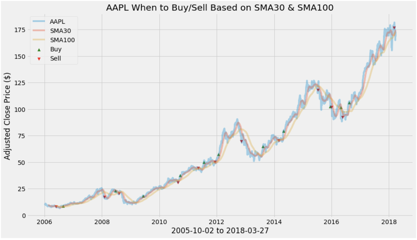
• As you can see the tick marks are not perfect because between 2008 and 2010 period, you can see the program actually sold it a lower price.
• However, in the long term, I decided that this will give a sufficient profit.

Full Code:

import numpy as np
from datetime import datetime
import matplotlib.pyplot as plt
plt.style.use("fivethirtyeight")

#loading the data
import quandl
quandl.ApiConfig.api_key = "Wdq5f9Fa6Pq-h5zJjR5w"
data = quandl.get("WIKI/AAPL", start_date="2006-01-01", end_date="2020-10-30")

SMA30 = pd.DataFrame()
SMA30['Adj. Close'] = data['Adj. Close'].rolling(window=30).mean()

SMA100 = pd.DataFrame()
SMA100['Adj. Close'] = data['Adj. Close'].rolling(window=100).mean()

# Calculating the average of volue of window of 50 days
VOL50 = pd.DataFrame()
VOL50['Adj. Volume'] = data['Adj. Volume'].rolling(window=50).mean()

# Calculating the average of volue of window of 15 days average
VOL15 = pd.DataFrame()
VOL15['Adj. Volume'] = data['Adj. Volume'].rolling(window=15).mean()

# visualizing the data
plt.figure(figsize=(20,14.5))
plt.plot(data['Adj. Close'], label="AAPL")
plt.plot(SMA30['Adj. Close'], label="SMA30")
plt.plot(SMA100['Adj. Close'], label="SMA100")

plt.title("Apple Adjusted Close Prices History")
plt.xlabel("2006-01-01 to 2018-03-27")
plt.ylabel("Adjusted Close Price ($)")
plt.legend(loc="upper left")

# We're going to buy whenever SMA crosses the long-term average
# Anytime SMA30 crosses the SMA100 will be the signal to buy!!
buy = pd.DataFrame()
buy['AAPL'] = data['Adj. Close']
buy['SMA30'] = SMA30['Adj. Close']
buy['SMA100'] = SMA100['Adj. Close']
buy['VOL15'] = VOL15['Adj. Volume']
buy['VOL50'] = VOL50['Adj. Volume']

# Function that tells you when to sell/buy
def buy_sell(data):
    sigBuy = []
    sigSell = []
    flag = -1
    for i in range(len(data)):
        # GOLDEN CROSS & VOL50 > VOL200
        if ((data['SMA30'][i] > data['SMA100'][i]) and (data['VOL15'][i] > data['VOL50'][i])):
            if flag != 1:
                sigBuy.append(data['AAPL'][i])
                sigSell.append(np.nan)
                flag = 1
            else:
                sigBuy.append(np.nan)
                sigSell.append(np.nan)
        # DEATH CROSS
        elif data['SMA30'][i] < data['SMA100'][i]:
            if flag != 0:
                sigBuy.append(np.nan)
                sigSell.append(data['AAPL'][i])
                flag = 0 
            else:
                sigBuy.append(np.nan)
                sigSell.append(np.nan)
        else:
            sigBuy.append(np.nan)
            sigSell.append(np.nan)
    return [sigBuy, sigSell]

buy_or_sell = buy_sell(buy)
buy['Signal to Buy'] = buy_or_sell[0]
buy['Signal to Sell'] = buy_or_sell[1]

# Visualize the data and strategize 
plt.figure(figsize=(14,8))
plt.plot(buy['AAPL'], label = "AAPL", alpha=0.35)
plt.plot(buy['SMA30'], label = "SMA30", alpha=0.35)
plt.plot(buy['SMA100'], label = "SMA100", alpha=0.35)
plt.scatter(buy.index, buy['Signal to Buy'], label ="Buy", marker ="^", color='green')
plt.scatter(buy.index, buy['Signal to Sell'], label ="Sell", marker ="v", color='red')
plt.title('AAPL When to Buy/Sell Based on SMA30 & SMA100')
plt.xlabel("2005-10-02 to 2018-03-27")
plt.ylabel("Adjusted Close Price ($)")
plt.legend(loc="upper left")

In the next blog, I'm going to backtest this startegy with "backtrader" module.

Thanks for reading :)