들어가며

Causal model은 causal quantities를 확인하기 위해 필수적이다. 이전 내용에서는 Causal model에 대한 graphical intuition을 확인했다. 이번 글에서는 더 나아가 두 가지 내용에 대해 설명할 예정이다.

1. Indentify causal quantities
2. Formalize causal models

---

4.1 $do$-operator and Interventional Distributions

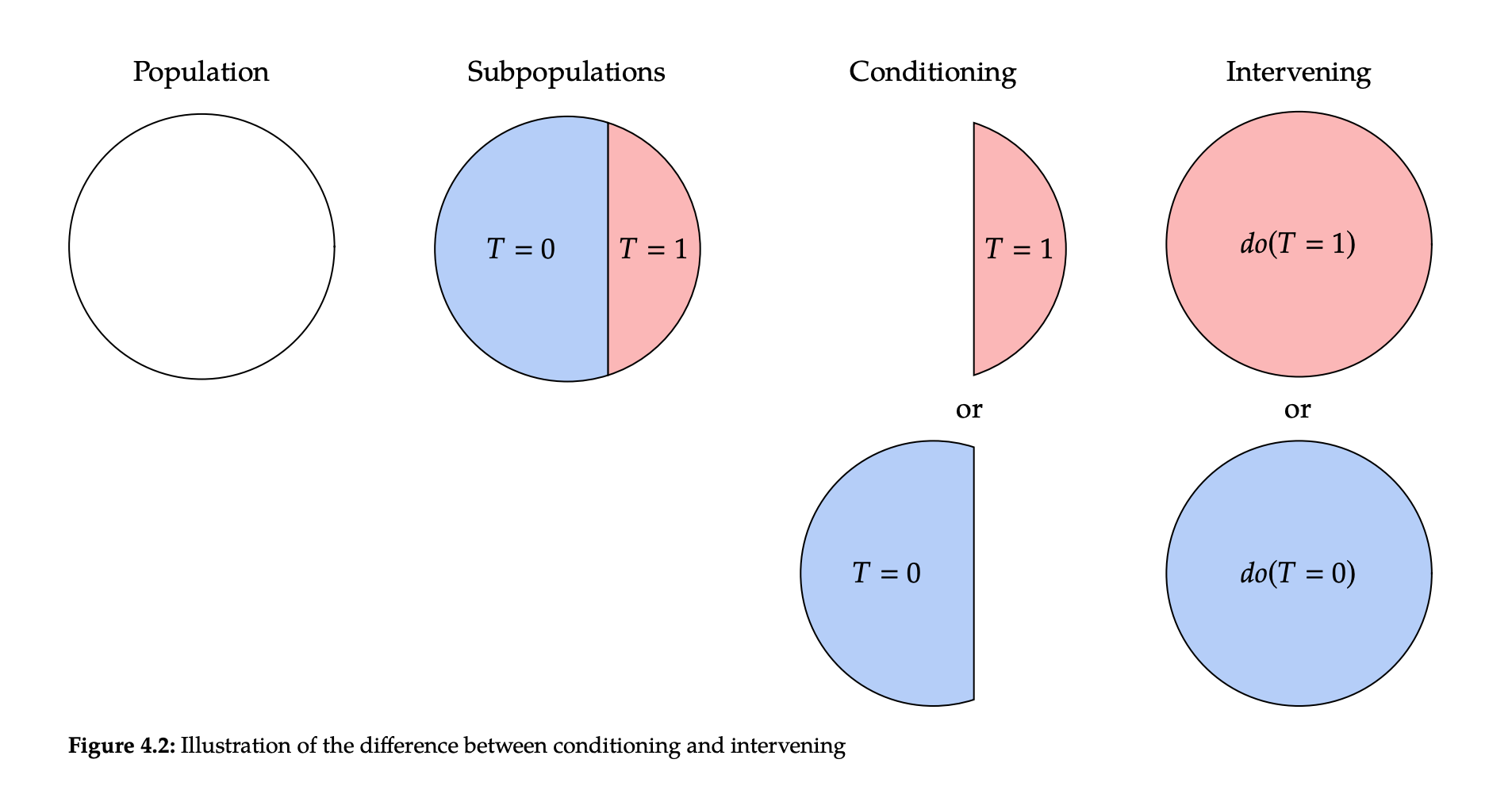
일반적으로 확률에 대한 계산을 할 때, 우리는 조건부 확률 (conditional probability)을 흔하게 접할 수 있다. 그러나 이렇게 conditioning을 하는 것과 intervening을 하는 것은 전혀 다른 이야기다. $T=t$ 라는 conditioning을 진행하는 것은, 단순하게 treatment t를 부여받은 분포에만 관심을 가지겠다는 뜻이다. 우린 앞으로 intervention을 표현할 때 $do$-operator를 활용할 것이다. 다음과 같이 표현한다.

$do(T=t)$

Conditioning on $T=t$ 는 전체 모집단 혹은 관측한 데이터에서 treatment t를 부여받은 subset이 된다.
Intervention on $T=t$ 는 전제 모집단에 대해 $T=t$ 로 생각한다는 뜻이다. 즉, Observation이 아닌 Doing(intervention)을 통해 인과관계를 도출하기 위한 과정 중 하나라고 생각 할 수 있다. 아래 그림을 통해 더 직관적으로 이해할 수 있다.

Observational distribution에 대해,
$P(Y), P(Y,T,X)$ 로 표현 가능 하다.

Interventional distribution의 경우,
$P(Y|do(T=t)), P(Y|do(T=t), X=x)$ 로 표현 가능하다.

$do$-operator를 통해 얻은 Causal effect를 Causal Estimand 라고 부르며, 그렇지 않은 관측치들에 대해서는 Statistical Estimand 라고 부른다. Identification의 가정하에, 우리는 Causal Estimand를 Statistical Estimand로 바꿀 수 있다. Treatment에 영향을 줄 수 있는 모든 변수의 효과를 무시하게 만들어주는게 바로 이 $do$ 연산자다.

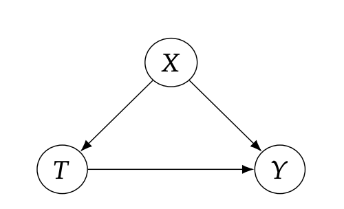
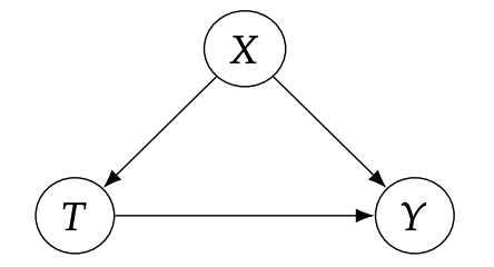
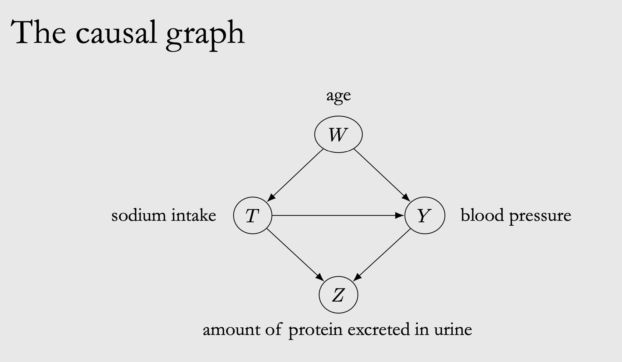
위 그래프에서 인과관계를 살펴보자. 만약, $X$ 노드가 존재하지 않았다면 $P(Y|T)$ 를 통해 인과효과를 파악할 수 있었을 것이다. 하지만 Confounder인 $X$ 의 존재로 인해, Backdoor path가 생기게 되어 인과효과를 파악하기 어려워진다. 여기서 $do$-operator가 빛을 발휘한다. 바로 그래프 내의 $X$ 와 $T$ 를 잇는 edge를 삭제할 수 있게 된다는 점이다.

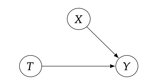
이런 그래프가 되는 것이다. $do(T=t)$ 가 적용되었다고 생각하면 된다. 우리는 $P(Y|do(T))$ 를 얻게 되며, 이 값이 바로 Causal effect라고 할 수 있다.

---

4.2 Main Assumption: Modularity

Causal Inference를 위해서는 정말 많은 가정들이 기반이 되어야 한다. 앞에서 계속 다뤘던 것처럼, interventions에 대해서도 'interventions are local' 이라는 가정이 들어가게 된다. Intervention node $X_i$ 에 대해서 $pa_i$ 가 미치는 영향에만 변화가 생기고 나머지 노드에서 받는 영향은 유지된다는 가정이다. 지금부터 다룰 Modularity assumption은 바로 이 'Inventions are local' 을 일반화한 가정이라고 생각하면 된다. 가정은 다음과 같다.

Assumption Modularity
If we intervene on a set of nodes $S\subseteq \ [n]$, setting them to constants, then for all $i$, we have the following:
1. If $i \notin\ S$, then $P(x_i|pa_i)$ remains unchaged.
2. If $i\in S$, then $P(x_i|pa_i)=1$ if $x_i$ is the value that $X_i$ was set to by the intervention; otherwise, $P(x_i|pa_i)=0$.

즉, 우리는 $P(Y)$, $P(Y|do(T=t))$, $P(Y|do(T_2=t_2))$가 서로 연관되지 않은 distribution임을 알 수 있다.

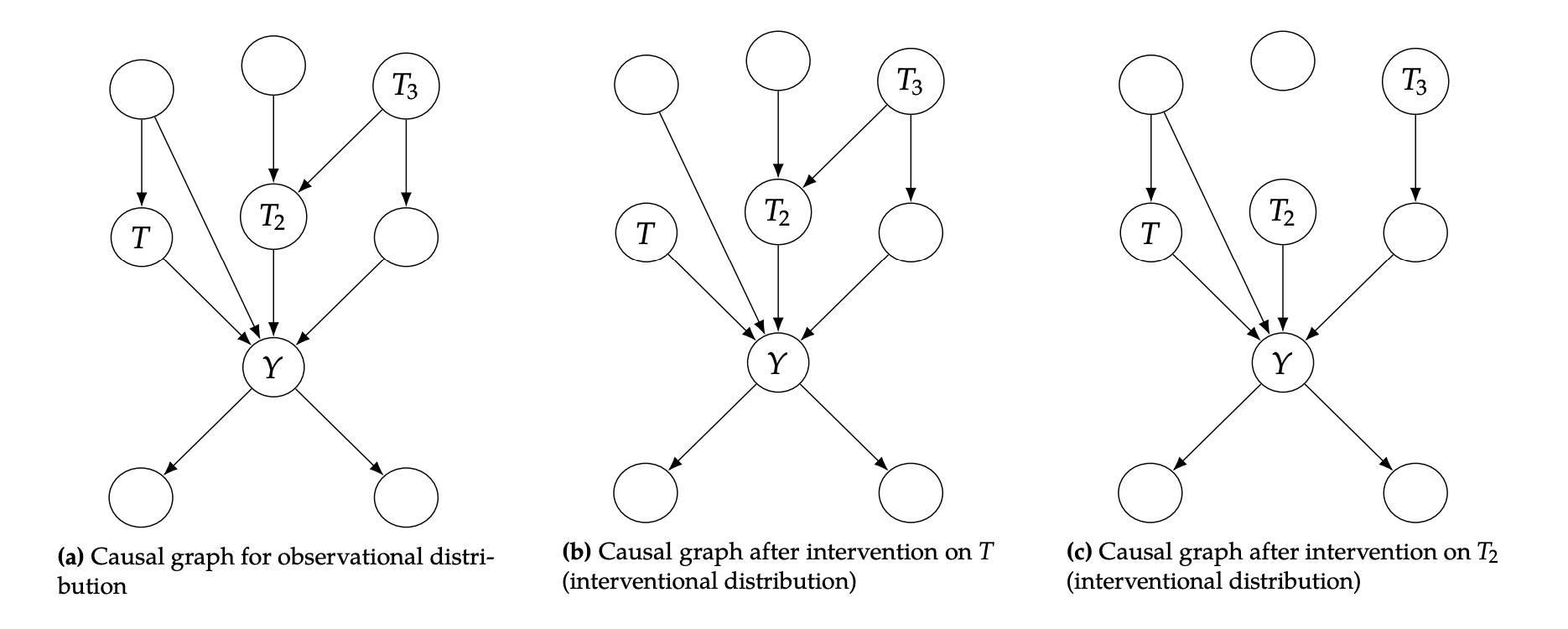
위 그림에서의 (b)와 (c)같이 edge가 제거된 그래프를 Manipulated graph라고 한다.

---

4.3 Truncated Factorization

앞에서 다룬 Bayesian network factorization을 떠올려보자.

$P(x_1,...,x_n)=\underset{i}{\Pi}P(x_i|pa_i)$

여기서 Modularity assumption을 적용할 수 있다. Intervention이 적용된 nodes set $S$ 에 포함되는 노드들은, $P(x_i|pa_i)=1$ 이 되어버리기 때문에, factorization에서 생략할 수 있다.

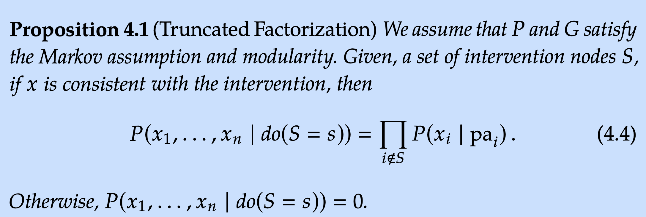
위와 같은 식이 도출된다.

위 그래프에 대해 $P(y|do(t)$ 를 통해,

Bayesian network factorization: $P(y,t,x)=P(x)P(t|x)P(y|t,x)$
Truncated factorization: $P(y,x,|do(t))=P(x)P(y|t,x)$
Marginalize: $P(y|do(t))=\underset{x}{\Sigma}P(y|t,x)P(x)$

를 확인 가능하다.

---

4.4 Backdoor Adjustment

이전 챕터에서 다뤘던 내용 처럼 backdoor path를 막는 것은 인과관계를 도출하기 위해 필수적이다. 이전 챕터에서는 conditioning을 통해 임의로 path를 차단하면서 potential outcome을 도출해 냈다. 이번 챕터에서는 $do$-operator를 통해 edge 자체를 삭제함과 동시에 backdoor path를 없애는 방식으로 optential outcome을 도출한다.
먼저, Backdoor Adjustment에 대해서 알아야 한다.

Backdoor Adjustment
Given the modularity assumption, that $W$ satisfies the backdoor criterion, and positivity, we can identify the causal effect of $T$ on $Y$:
$P(y|do(t))=\underset{w}{\Sigma}P(y|t,w)P(w)$

Proof of backdoor adjustment
$P(y|do(t))=\underset{w}{\Sigma}P(y|do(t),w)P(w|do(t))$
$=\underset{w}{\Sigma}P(y|t,w)P(w|do(t))$
$=\underset{w}{\Sigma}P(y|t,w)P(w)$

여기서 드는 의문점이 있다. Conditioning을 통한 Potential outcome과 backdoor adjustment를 통해 얻을 수 있는 결과값이 같다면, 왜 굳이 $do$-operator를 통해 backdoor path를 막는 것인지 의문이 든다. 뭐, chapter 14에서 더 자세하게 다룬다고는 하니까 믿고 기다려보기로 한다...

---

4.5 Structural Causal Models (SCMs)

지금까지 다룬 내용을 Structural causal model로 만들었다고 이해하면 된다. 인과관계에서는 역이 성립하지 않는다. 다시 말해, $A=B$ 라고 해서 $B=A$가 인과관계에서는 성립하지 않는다.
그래서 다음과 같은 notation을 사용한다.

$B:=f(A,U)$

위 수식은 아래 그림에 대한 내용이다.

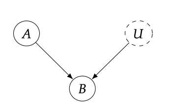
이 수식을 좀 더 확장해서 다음과 같은 그래프에 대해서 표현 할 수 있다.

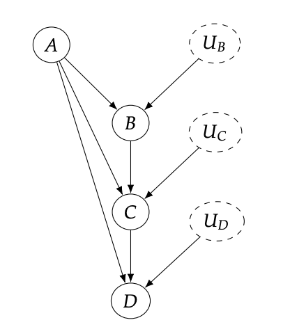
위 그래프에 대해서 우리는

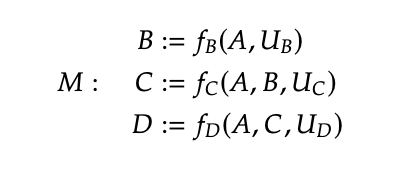
이렇게 표현 할 수 있다.

Collider의 경우 앞에서 다뤘던 것 처럼, block 하는 순간 부모 노드들 사이의 independent가 없어지게 된다. 그렇기에 SCMs에서도 collider에 유의해야 한다.

$T:=f_T(X,U_T)$
$Y:=f_Y(X,T,U_Y)$

에 대해서 intervention on $T$ 를 진행하면 다음과 같이 표현 된다.

$T:=t$
$Y:=f_Y(X,T,U_Y)$

---

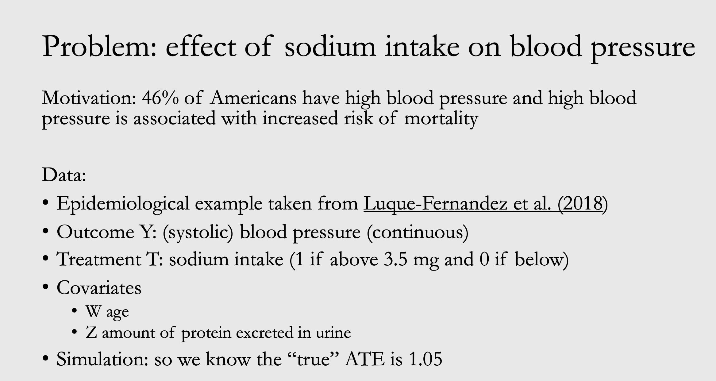
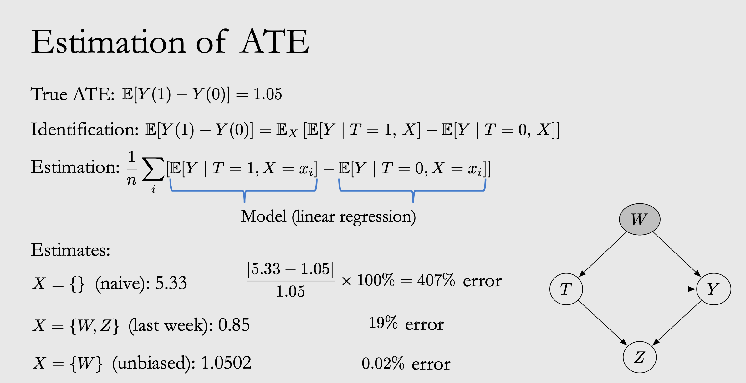
4.6 Example Application of Backddor Adjustment

"""
Estimating the causal effect of sodium on blood pressure in a simulated example
adapted from Luque-Fernandez et al. (2018):
    https://academic.oup.com/ije/article/48/2/640/5248195
"""

import numpy as np
import pandas as pd
from sklearn.linear_model import LinearRegression


def generate_data(n=1000, seed=0, beta1=1.05, alpha1=0.4, alpha2=0.3, binary_treatment=True, binary_cutoff=3.5):
    np.random.seed(seed)
    age = np.random.normal(65, 5, n)
    sodium = age / 18 + np.random.normal(size=n)
    if binary_treatment:
        if binary_cutoff is None:
            binary_cutoff = sodium.mean()
        sodium = (sodium > binary_cutoff).astype(int)
    blood_pressure = beta1 * sodium + 2 * age + np.random.normal(size=n)
    proteinuria = alpha1 * sodium + alpha2 * blood_pressure + np.random.normal(size=n)
    hypertension = (blood_pressure >= 140).astype(int)  # not used, but could be used for binary outcomes
    return pd.DataFrame({'blood_pressure': blood_pressure, 'sodium': sodium,
                         'age': age, 'proteinuria': proteinuria})


def estimate_causal_effect(Xt, y, model=LinearRegression(), treatment_idx=0, regression_coef=False):
    model.fit(Xt, y)
    if regression_coef:
        return model.coef_[treatment_idx]
    else:
        Xt1 = pd.DataFrame.copy(Xt)
        Xt1[Xt.columns[treatment_idx]] = 1
        Xt0 = pd.DataFrame.copy(Xt)
        Xt0[Xt.columns[treatment_idx]] = 0
        return (model.predict(Xt1) - model.predict(Xt0)).mean()


if __name__ == '__main__':
    binary_t_df = generate_data(beta1=1.05, alpha1=.4, alpha2=.3, binary_treatment=True, n=10000000)
    continuous_t_df = generate_data(beta1=1.05, alpha1=.4, alpha2=.3, binary_treatment=False, n=10000000)

    ate_est_naive = None
    ate_est_adjust_all = None
    ate_est_adjust_age = None

    for df, name in zip([binary_t_df, continuous_t_df],
                        ['Binary Treatment Data', 'Continuous Treatment Data']):
        print()
        print('### {} ###'.format(name))
        print()

        # Adjustment formula estimates
        ate_est_naive = estimate_causal_effect(df[['sodium']], df['blood_pressure'], treatment_idx=0)
        ate_est_adjust_all = estimate_causal_effect(df[['sodium', 'age', 'proteinuria']],
                                                    df['blood_pressure'], treatment_idx=0)
        ate_est_adjust_age = estimate_causal_effect(df[['sodium', 'age']], df['blood_pressure'])
        print('# Adjustment Formula Estimates #')
        print('Naive ATE estimate:\t\t\t\t\t\t\t', ate_est_naive)
        print('ATE estimate adjusting for all covariates:\t', ate_est_adjust_all)
        print('ATE estimate adjusting for age:\t\t\t\t', ate_est_adjust_age)
        print()

        # Linear regression coefficient estimates
        ate_est_naive = estimate_causal_effect(df[['sodium']], df['blood_pressure'], treatment_idx=0,
                                               regression_coef=True)
        ate_est_adjust_all = estimate_causal_effect(df[['sodium', 'age', 'proteinuria']],
                                                    df['blood_pressure'], treatment_idx=0,
                                                    regression_coef=True)
        ate_est_adjust_age = estimate_causal_effect(df[['sodium', 'age']], df['blood_pressure'],
                                                    regression_coef=True)
        print('# Regression Coefficient Estimates #')
        print('Naive ATE estimate:\t\t\t\t\t\t\t', ate_est_naive)
        print('ATE estimate adjusting for all covariates:\t', ate_est_adjust_all)
        print('ATE estimate adjusting for age:\t\t\t\t', ate_est_adjust_age)
        print()