블록과 함께하는 파이썬 딥러닝 케라스

김경민·2022년 6월 7일

AI

목록 보기

3/11

conda create -n deep python=3.7 
conda activate deep 
pip install tensorflow==2.0

인공지능 > 머신러닝 > 딥러닝

기계학습

기존의 코딩

-> 조건을 라인바이라인으로 긴 코드로 써내려 가는 일

앞으로의 코딩

-> 조건을 학습 도델의 여러 가중치로 변환하는 일

머신러닝

-> 가르쳐주는 학습 -> 분류, 회귀

-> 자율학습 -> 군집

지도학습 - KNN ( k Nearest Neighbors ) : 최근접 이웃 알고리즘

import random
import numpy as np

r=[] # 여자 1
b=[] # 남자 0

for i in range(50):
r.append([random.randint(40, 70), random.randint(140, 180), 1])
b.append([random.randint(60, 90), random.randint(160, 200), 0])

def distance(x,y):
#두 점 사이의 거리를 구하는 함수
return np.sqrt(pow((x[0]-y[0]),2) + pow((x[1]-y[1]),2))

def knn(x,y,k):

result=[]
cnt=0

for i in range(len(y)):
result.append([distance(x,y[i]),y[i][2]])
result.sort()

for i in range(k):
if(result[i][1]==1):
cnt += 1

if (cnt > (k/2)):
print ("당신은 여자입니다.")
else:
print ("당신은 남자입니다.")

weight = input("몸무게를 입력해 주세요. ")
height = input("키를 입력해 주세요. ")
num = input("k를 입력해 주세요. ")

new = [int(weight), int(height)]
knn(new, r+b, int(num))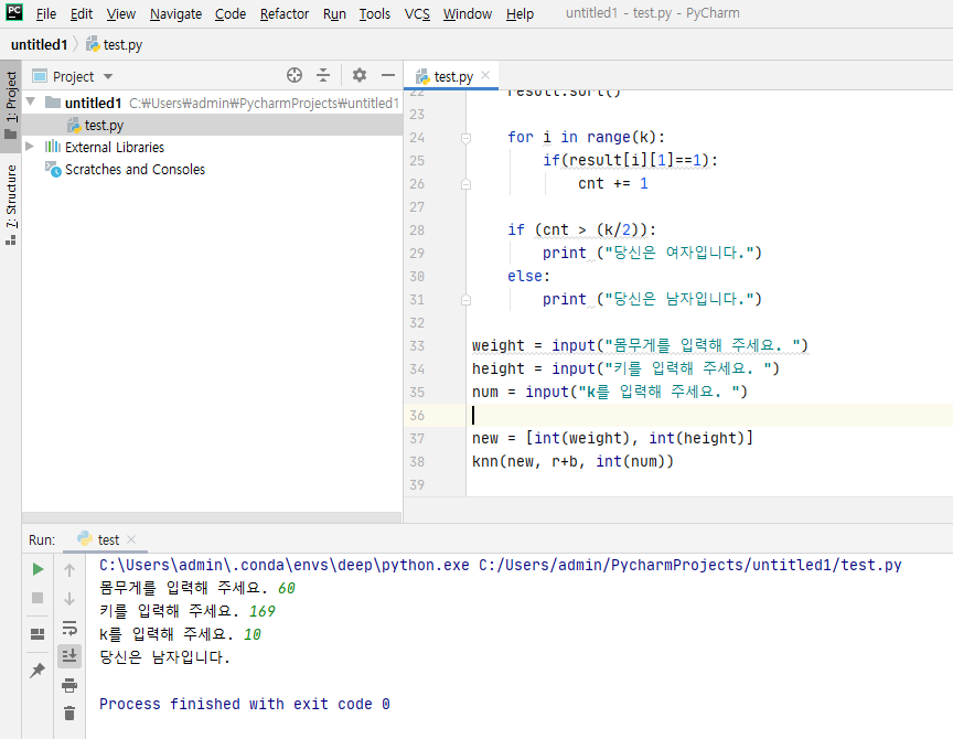

pip install matplotlib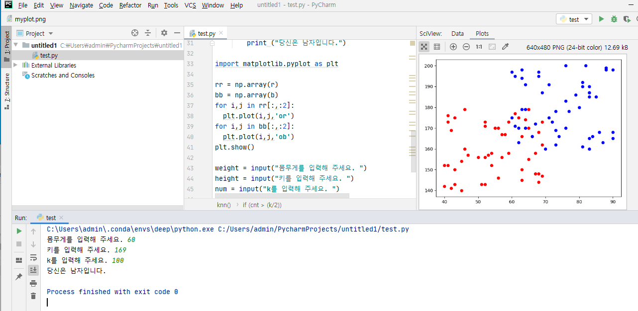

import random
import numpy as np

r=[] # 여자 1
b=[] # 남자 0

for i in range(50):
r.append([random.randint(40, 70), random.randint(140, 180), 1])
b.append([random.randint(60, 90), random.randint(160, 200), 0])

def distance(x,y):
#두 점 사이의 거리를 구하는 함수
return np.sqrt(pow((x[0]-y[0]),2) + pow((x[1]-y[1]),2))

def knn(x,y,k):

result=[]
cnt=0

for i in range(len(y)):
result.append([distance(x,y[i]),y[i][2]])
result.sort()

for i in range(k):
if(result[i][1]==1):
cnt += 1

if (cnt > (k/2)):
print ("당신은 여자입니다.")
else:
print ("당신은 남자입니다.")

import matplotlib.pyplot as plt

rr = np.array(r)
bb = np.array(b)
for i,j in rr[:,:2]:
plt.plot(i,j,'or')
for i,j in bb[:,:2]:
plt.plot(i,j,'ob')
plt.show()

weight = input("몸무게를 입력해 주세요. ")
height = input("키를 입력해 주세요. ")
num = input("k를 입력해 주세요. ")

new = [int(weight), int(height)]
knn(new, r+b, int(num))

딥러닝

사람의 뇌세포와 가상의 모델 - 인공신경망

매우 많은 Hidden Layers = Deep

수확가속의 법칙, 무어의 법칙

합성곱 신경망 (Convolutional Neural Network, CNN)
순환 신경망 (Recurrent Neural Network, RNN)

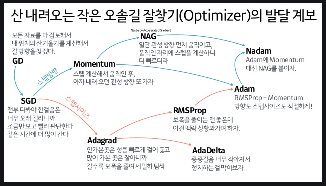
옵티마이저: Gradient Decent
활성화 함수
Batch 학습
DropOut
LearningRate
순전파, 역전파

- 텐서플로우2.0 케라스

-> 데이터셋 생성

-> 모델구성

-> 모델 학습 과정 설정

-> 모델학습

-> 학습과정

-> 모델평가

-> 모델사용

데이터 셋

-> 훈련셋, 시험셋, 실전

-> 훈련셋, 검증셋, 시험셋, 실전

epochs
Model.fit()
EarlyStopping

성능평가지표: 정확도, 정밀도, 재현율, Accuracy, Precision, Recall

A, B 의사 중 A의사는 암환자를 100% 찾음, B의사는 50% 찾음, A의사는 진료한 모든 환자에게 암진단, B의사는 암으로 진단한 환자는 100% 암환자

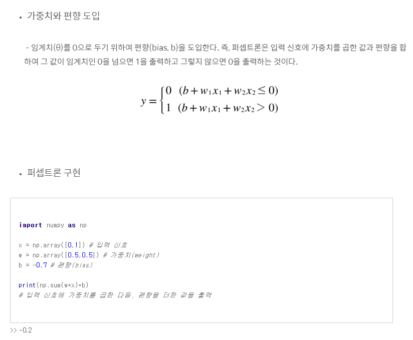
* 퍼셉트론

다수의 신호를 입력으로 받아 하나의 신호를 출력
퍼셉트론 신호는 흐름을 만들고 정보를 앞으로 전달한다.
퍼셉트론 신호는 '흐른다/안 흐른다' 두 가지의 값을 가진다.

* 다층 퍼셉트론

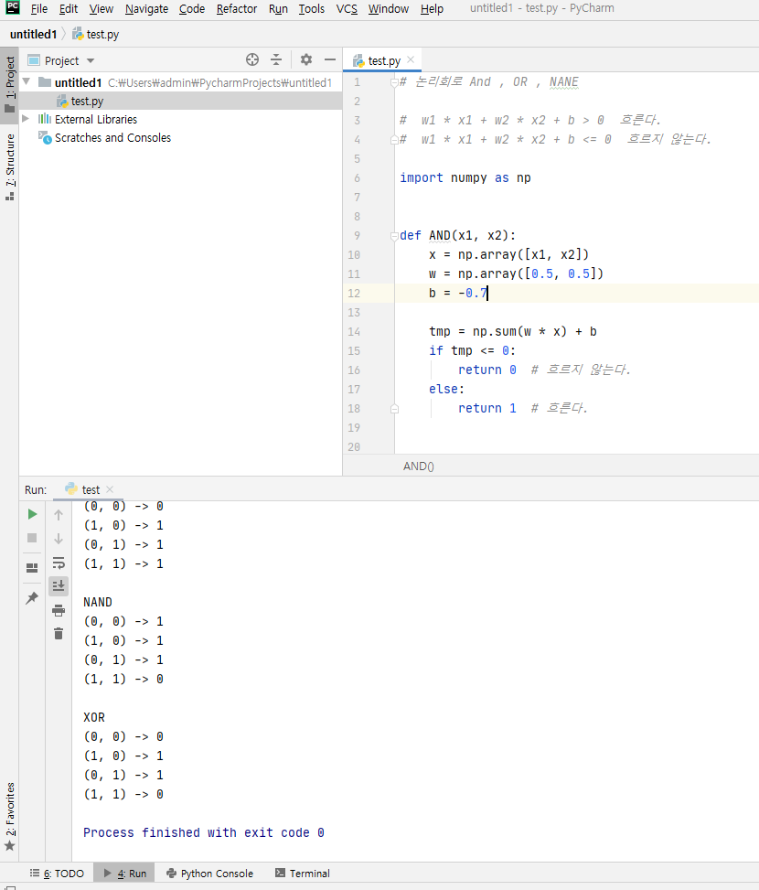
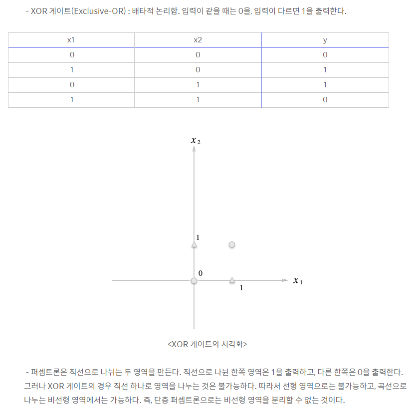
논리회로 And , OR , NANE

w1 x1 + w2 x2 + b > 0 흐른다.

w1 x1 + w2 x2 + b <= 0 흐르지 않는다.

import numpy as np


def AND(x1, x2):
x = np.array([x1, x2])
w = np.array([0.5, 0.5])
b = -0.7

tmp = np.sum(w * x) + b
if tmp <= 0:
return 0 # 흐르지 않는다.
else:
return 1 # 흐른다.


def OR(x1, x2):
x = np.array([x1, x2])
w = np.array([0.5, 0.5])
b = -0.2

tmp = np.sum(w * x) + b
if tmp <= 0:
return 0 # 흐르지 않는다.
else:
return 1 # 흐른다.


def NAND(x1, x2):
x = np.array([x1, x2])
w = np.array([-0.5, -0.5])
b = 0.7

tmp = np.sum(w * x) + b
if tmp <= 0:
return 0 # 흐르지 않는다.
else:
return 1 # 흐른다.


print("AND")
for i in [(0, 0), (1, 0), (0, 1), (1, 1)]:
y = AND(i[0], i[1])
print(str(i) + " -> " + str(y))
print()
print("OR")
for i in [(0, 0), (1, 0), (0, 1), (1, 1)]:
y = OR(i[0], i[1])
print(str(i) + " -> " + str(y))
print()
print("NAND")
for i in [(0, 0), (1, 0), (0, 1), (1, 1)]:
y = NAND(i[0], i[1])
print(str(i) + " -> " + str(y))

print()
print("XOR")
for i in [(0, 0), (1, 0), (0, 1), (1, 1)]:
s1 = NAND(i[0], i[1])
s2 = OR(i[0], i[1])
y = AND(s1, s2)

print(str(i) + " -> " + str(y))

* 다층 퍼셉트론 레이어

순전파(Feedforward)
역전파(Backpropagation)

Dense(8, input_dim=4, init='uniform', activation='relu'), 크고 낮을수록 미치는 영향이 적다.

첫번째 인자: 출력 뉴런의 수를 설정
input_dim: 입력 뉴런의 수를 설정
init: 가중치 초기화 방법 설정, 'uniform': 균일 분포, 'normal': 가우시안 분포
activation: 활성화 함수 설정, 'linear', 'relu', 'sigmoid': 시그모이드 함수, 이진 분류 문제에 출력층에 주로 쓰임, 'softmax': 소프트맥스 함수, 다중 클래스 분류 출력층에 주로 쓰임

!pip install tensorflow==2.0

# Commented out IPython magic to ensure Python compatibility.
import tensorflow as tf
# print(tf.__version__)
import tensorflow.keras.utils as utils
from tensorflow.keras.datasets import mnist
from tensorflow.keras.models import Sequential
from tensorflow.keras.layers import Dense, Activation
import numpy as np
import matplotlib.pyplot as plt
# %matplotlib inline

데이터셋 준비하기

X_train = np.array(
[
1,2,3,4,5,6,7,8,9,1,2,3,4,5,6,7,8,9,1,2,3,4,5,6,7,8,9,1,2,3,4,5,6,7,8,9,1,2,3,4,5,6,7,8,9,1,2,3,4,5,6,7,8,9,1,2,3,4,5,6,7,8,9,1,2,3,4,5,6,7,8,9,1,2,3,4,5,6,7,8,9,1,2,3,4,5,6,7,8,9,1,2,3,4,5,6,7,8,9,1,2,3,4,5,6,7,8,9,1,2,3,4,5,6,7,8,9,1,2,3,4,5,6,7,8,9,1,2,3,4,5,6,7,8,9,1,2,3,4,5,6,7,8,9,1,2,3,4,5,6,7,8,9,1,2,3,4,5,6,7,8,9,1,2,3,4,5,6,7,8,9,1,2,3,4,5,6,7,8,9,1,2,3,4,5,6,7,8,9
]
)

Y_train = np.array(
[
2,4,6,8,10,12,14,16,18,2,4,6,8,10,12,14,16,18,2,4,6,8,10,12,14,16,18,2,4,6,8,10,12,14,16,18,2,4,6,8,10,12,14,16,18,2,4,6,8,10,12,14,16,18,2,4,6,8,10,12,14,16,18,2,4,6,8,10,12,14,16,18,2,4,6,8,10,12,14,16,18,2,4,6,8,10,12,14,16,18,2,4,6,8,10,12,14,16,18,2,4,6,8,10,12,14,16,18,2,4,6,8,10,12,14,16,18,2,4,6,8,10,12,14,16,18,2,4,6,8,10,12,14,16,18,2,4,6,8,10,12,14,16,18,2,4,6,8,10,12,14,16,18,2,4,6,8,10,12,14,16,18,2,4,6,8,10,12,14,16,18,2,4,6,8,10,12,14,16,18,2,4,6,8,10,12,14,16,18
])

X_val = np.array(
[
1,2,3,4,5,6,7,8,9,1,2,3,4,5,6,7,8,9,1,2,3,4,5,6,7,8,9
])

Y_val = np.array(
[
2,4,6,8,10,12,14,16,18,2,4,6,8,10,12,14,16,18,2,4,6,8,10,12,14,16,18
])

라벨링 전환

Y_train = utils.to_categorical(Y_train,19)
Y_val = utils.to_categorical(Y_val,19)


model = Sequential()
model.add(Dense(units=38, input_dim=1, activation='elu'))
model.add(Dense(units=19, activation='softmax'))

model.compile(loss='categorical_crossentropy', optimizer='sgd', metrics=['accuracy'])

모델 학습시키기

hist = model.fit(X_train, Y_train, epochs=200, batch_size=1, verbose=0, validation_data=(X_val, Y_val))

fig, loss_ax = plt.subplots()

acc_ax = loss_ax.twinx()

loss_ax.plot(hist.history['loss'], 'y', label='train loss')
loss_ax.plot(hist.history['val_loss'], 'r', label='val loss')

acc_ax.plot(hist.history['accuracy'], 'b', label='train acc')
acc_ax.plot(hist.history['val_accuracy'], 'g', label='val acc')

loss_ax.set_xlabel('epoch')
loss_ax.set_ylabel('loss')
acc_ax.set_ylabel('accuray')

loss_ax.legend(loc='upper left')
acc_ax.legend(loc='lower left')

plt.show()

# 6. 모델 사용하기
X_test = np.array([
1, 2, 3, 4, 5, 6, 7, 8, 9
])
Y_test = np.array([
[0, 0, 1, 0, 0, 0, 0, 0, 0, 0, 0, 0, 0, 0, 0, 0, 0, 0, 0],
[0, 0, 0, 0, 1, 0, 0, 0, 0, 0, 0, 0, 0, 0, 0, 0, 0, 0, 0],
[0, 0, 0, 0, 0, 0, 1, 0, 0, 0, 0, 0, 0, 0, 0, 0, 0, 0, 0],
[0, 0, 0, 0, 0, 0, 0, 0, 1, 0, 0, 0, 0, 0, 0, 0, 0, 0, 0],
[0, 0, 0, 0, 0, 0, 0, 0, 0, 0, 1, 0, 0, 0, 0, 0, 0, 0, 0],
[0, 0, 0, 0, 0, 0, 0, 0, 0, 0, 0, 0, 1, 0, 0, 0, 0, 0, 0],
[0, 0, 0, 0, 0, 0, 0, 0, 0, 0, 0, 0, 0, 0, 1, 0, 0, 0, 0],
[0, 0, 0, 0, 0, 0, 0, 0, 0, 0, 0, 0, 0, 0, 0, 0, 1, 0, 0],
[0, 0, 0, 0, 0, 0, 0, 0, 0, 0, 0, 0, 0, 0, 0, 0, 0, 0, 1]

])
loss_and_metrics = model.evaluate(X_test, Y_test, batch_size=1)

print('')
print('loss : ' + str(loss_and_metrics[0]))
print('accuray : ' + str(loss_and_metrics[1]))

# Commented out IPython magic to ensure Python compatibility.
import tensorflow as tf
# print(tf.__version__)
import tensorflow.keras.utils as utils
from tensorflow.keras.datasets import mnist
from tensorflow.keras.models import Sequential
from tensorflow.keras.layers import Dense, Activation
import numpy as np
import matplotlib.pyplot as plt
import random
# %matplotlib inline
x_data = []
for i in range(100):
x_data.append([random.randint(40, 60),random.randint(140, 170)])
x_data.append([random.randint(60, 90),random.randint(170, 200)])
y_data = []
for i in range(100):
y_data.append(1)#여
y_data.append(0)#남
# 1. 데이터셋 준비하기
X_train = np.array([x_data])
X_train = X_train.reshape(200,2)

Y_train = np.array(y_data)
Y_train = Y_train.reshape(200,)



print(X_train[0])
print(Y_val[0])

model = Sequential()
model.add(Dense(20, input_dim=2, activation='relu'))
model.add(Dense(10, activation='relu'))
model.add(Dense(1, activation='sigmoid'))

model.compile(loss='binary_crossentropy', optimizer='adam', metrics=['accuracy'])

모델 학습시키기

hist = model.fit(X_train, Y_train, epochs=200, batch_size=10, verbose=1)


fig, loss_ax = plt.subplots()

acc_ax = loss_ax.twinx()

loss_ax.plot(hist.history['loss'], 'y', label='train loss')
# loss_ax.plot(hist.history['val_loss'], 'r', label='val loss')

acc_ax.plot(hist.history['accuracy'], 'b', label='train acc')
# acc_ax.plot(hist.history['val_accuracy'], 'g', label='val acc')

loss_ax.set_xlabel('epoch')
loss_ax.set_ylabel('loss')
acc_ax.set_ylabel('accuray')

loss_ax.legend(loc='upper left')
acc_ax.legend(loc='lower left')

plt.show()

x_test = np.array([[50,150],[80,180],[75,170],[60,150],[45,155]])
x_test = x_test.reshape(5,2)
y_test = np.array([1,0,0,1,1])
scores = model.evaluate(x_test, y_test)
print("%s: %.2f%%" %(model.metrics_names[1], scores[1]*100))

x_data = []
for i in range(20):
x_data.append([random.randint(40, 60),random.randint(140, 170)])
x_data.append([random.randint(60, 90),random.randint(170, 200)])
y_data = []
for i in range(20):
y_data.append(1)#여
y_data.append(0)#남
# 1. 데이터셋 준비하기
x_test = np.array([x_data])
x_test = x_test.reshape(40,2)

y_test = np.array(y_data)
y_test = y_test.reshape(40,)

yhat = model.predict_classes(x_test)
for i in range(len(x_test)):
print(x_test[i])
print('True : ' + str(y_test[i]) + ', Predict : ' + str(yhat[i]))
print()

============= result ===============



9/1 [==============================================================================================================================================================================================================================================================================] - 0s 7ms/sample - loss: 0.0889 - accuracy: 1.0000 

loss : 0.1424690584341685 
accuray : 1.0 
[ 58 149] 
[0. 0. 1. 0. 0. 0. 0. 0. 0. 0. 0. 0. 0. 0. 0. 0. 0. 0. 0.] 
Train on 200 samples 
Epoch 1/200 

 10/200 [>.............................] - ETA: 4s - loss: 16.2614 - accuracy: 0.5000 
200/200 [==============================] - 0s 1ms/sample - loss: 6.5254 - accuracy: 0.4700 
Epoch 2/200 

 10/200 [>.............................] - ETA: 0s - loss: 4.5406 - accuracy: 0.2000 
200/200 [==============================] - 0s 156us/sample - loss: 1.0952 - accuracy: 0.5850 
Epoch 3/200 

 10/200 [>.............................] - ETA: 0s - loss: 0.7697 - accuracy: 0.5000 
200/200 [==============================] - 0s 78us/sample - loss: 0.6927 - accuracy: 0.5600 
Epoch 4/200 

 10/200 [>.............................] - ETA: 0s - loss: 0.3611 - accuracy: 1.0000 
200/200 [==============================] - 0s 78us/sample - loss: 0.5439 - accuracy: 0.7400 
Epoch 5/200 

 10/200 [>.............................] - ETA: 0s - loss: 0.5720 - accuracy: 0.6000 
200/200 [==============================] - 0s 78us/sample - loss: 0.5198 - accuracy: 0.7550 
Epoch 6/200 

 10/200 [>.............................] - ETA: 0s - loss: 0.4730 - accuracy: 0.7000 
200/200 [==============================] - 0s 78us/sample - loss: 0.5582 - accuracy: 0.6700 
Epoch 7/200 

 10/200 [>.............................] - ETA: 0s - loss: 0.4560 - accuracy: 0.8000 
200/200 [==============================] - 0s 78us/sample - loss: 0.5506 - accuracy: 0.6900 
Epoch 8/200 

 10/200 [>.............................] - ETA: 0s - loss: 0.7339 - accuracy: 0.6000 
200/200 [==============================] - 0s 78us/sample - loss: 0.4822 - accuracy: 0.7800 
Epoch 9/200 

 10/200 [>.............................] - ETA: 0s - loss: 0.4067 - accuracy: 0.9000 
200/200 [==============================] - 0s 78us/sample - loss: 0.4541 - accuracy: 0.7600 
Epoch 10/200 

 10/200 [>.............................] - ETA: 0s - loss: 0.4785 - accuracy: 0.8000 
200/200 [==============================] - 0s 78us/sample - loss: 0.4596 - accuracy: 0.7500 
Epoch 11/200 

 10/200 [>.............................] - ETA: 0s - loss: 0.4516 - accuracy: 0.6000 
200/200 [==============================] - 0s 156us/sample - loss: 0.4577 - accuracy: 0.7450 
Epoch 12/200 

 10/200 [>.............................] - ETA: 0s - loss: 0.3985 - accuracy: 0.7000 
200/200 [==============================] - 0s 78us/sample - loss: 0.4776 - accuracy: 0.7250 
Epoch 13/200 

 10/200 [>.............................] - ETA: 0s - loss: 0.3117 - accuracy: 1.0000 
200/200 [==============================] - 0s 78us/sample - loss: 0.4333 - accuracy: 0.7750 
Epoch 14/200 

 10/200 [>.............................] - ETA: 0s - loss: 0.4142 - accuracy: 0.8000 
200/200 [==============================] - 0s 78us/sample - loss: 0.4250 - accuracy: 0.8100 
Epoch 15/200 

 10/200 [>.............................] - ETA: 0s - loss: 0.6721 - accuracy: 0.5000 
200/200 [==============================] - 0s 78us/sample - loss: 0.4441 - accuracy: 0.7500 
Epoch 16/200 

 10/200 [>.............................] - ETA: 0s - loss: 0.4186 - accuracy: 0.8000 
200/200 [==============================] - 0s 78us/sample - loss: 0.4562 - accuracy: 0.7650 
Epoch 17/200 

 10/200 [>.............................] - ETA: 0s - loss: 0.4121 - accuracy: 0.9000 
200/200 [==============================] - 0s 156us/sample - loss: 0.5091 - accuracy: 0.7350 
Epoch 18/200 

 10/200 [>.............................] - ETA: 0s - loss: 0.4768 - accuracy: 0.8000 
200/200 [==============================] - 0s 78us/sample - loss: 0.4194 - accuracy: 0.7650 
Epoch 19/200 

 10/200 [>.............................] - ETA: 0s - loss: 0.4975 - accuracy: 0.8000 
200/200 [==============================] - 0s 78us/sample - loss: 0.4742 - accuracy: 0.7650 
Epoch 20/200 

 10/200 [>.............................] - ETA: 0s - loss: 0.3676 - accuracy: 0.8000 
200/200 [==============================] - 0s 78us/sample - loss: 0.4718 - accuracy: 0.7550 
Epoch 21/200 

 10/200 [>.............................] - ETA: 0s - loss: 0.4497 - accuracy: 0.6000 
200/200 [==============================] - 0s 78us/sample - loss: 0.5758 - accuracy: 0.7350 
Epoch 22/200 

 10/200 [>.............................] - ETA: 0s - loss: 0.4378 - accuracy: 0.8000 
200/200 [==============================] - 0s 78us/sample - loss: 0.4561 - accuracy: 0.7700 
Epoch 23/200 

 10/200 [>.............................] - ETA: 0s - loss: 0.3829 - accuracy: 0.8000 
200/200 [==============================] - 0s 78us/sample - loss: 0.4815 - accuracy: 0.7200 
Epoch 24/200 

 10/200 [>.............................] - ETA: 0s - loss: 0.4210 - accuracy: 0.8000 
200/200 [==============================] - 0s 78us/sample - loss: 0.4250 - accuracy: 0.7700 
Epoch 25/200 

 10/200 [>.............................] - ETA: 0s - loss: 0.5895 - accuracy: 0.7000 
200/200 [==============================] - 0s 78us/sample - loss: 0.4560 - accuracy: 0.7500 
Epoch 26/200 

 10/200 [>.............................] - ETA: 0s - loss: 0.4725 - accuracy: 0.6000 
200/200 [==============================] - 0s 156us/sample - loss: 0.4468 - accuracy: 0.7400 
Epoch 27/200 

 10/200 [>.............................] - ETA: 0s - loss: 0.4354 - accuracy: 0.8000 
200/200 [==============================] - 0s 78us/sample - loss: 0.4045 - accuracy: 0.7500 
Epoch 28/200 

 10/200 [>.............................] - ETA: 0s - loss: 0.3011 - accuracy: 0.8000 
200/200 [==============================] - 0s 78us/sample - loss: 0.4104 - accuracy: 0.7450 
Epoch 29/200 

 10/200 [>.............................] - ETA: 0s - loss: 0.4523 - accuracy: 0.7000 
200/200 [==============================] - 0s 78us/sample - loss: 0.4062 - accuracy: 0.7900 
Epoch 30/200 

 10/200 [>.............................] - ETA: 0s - loss: 0.3128 - accuracy: 0.8000 
200/200 [==============================] - 0s 78us/sample - loss: 0.4347 - accuracy: 0.7850 
Epoch 31/200 

 10/200 [>.............................] - ETA: 0s - loss: 0.0796 - accuracy: 1.0000 
200/200 [==============================] - 0s 78us/sample - loss: 0.4021 - accuracy: 0.8100 
Epoch 32/200 

 10/200 [>.............................] - ETA: 0s - loss: 0.4472 - accuracy: 0.7000 
200/200 [==============================] - 0s 156us/sample - loss: 0.4435 - accuracy: 0.7250 
Epoch 33/200 

 10/200 [>.............................] - ETA: 0s - loss: 0.4080 - accuracy: 0.8000 
200/200 [==============================] - 0s 78us/sample - loss: 0.4114 - accuracy: 0.7450 
Epoch 34/200 

 10/200 [>.............................] - ETA: 0s - loss: 0.5712 - accuracy: 0.6000 
200/200 [==============================] - 0s 78us/sample - loss: 0.4192 - accuracy: 0.7250 
Epoch 35/200 

 10/200 [>.............................] - ETA: 0s - loss: 0.3591 - accuracy: 0.7000 
200/200 [==============================] - 0s 78us/sample - loss: 0.5734 - accuracy: 0.7250 
Epoch 36/200 

 10/200 [>.............................] - ETA: 0s - loss: 0.3946 - accuracy: 0.7000 
200/200 [==============================] - 0s 78us/sample - loss: 0.5369 - accuracy: 0.7250 
Epoch 37/200 

 10/200 [>.............................] - ETA: 0s - loss: 0.1608 - accuracy: 1.0000 
200/200 [==============================] - 0s 78us/sample - loss: 0.4410 - accuracy: 0.7700 
Epoch 38/200 

 10/200 [>.............................] - ETA: 0s - loss: 0.3579 - accuracy: 0.7000 
200/200 [==============================] - 0s 78us/sample - loss: 0.4392 - accuracy: 0.7500 
Epoch 39/200 

 10/200 [>.............................] - ETA: 0s - loss: 0.2949 - accuracy: 0.8000 
200/200 [==============================] - 0s 78us/sample - loss: 0.4363 - accuracy: 0.7400 
Epoch 40/200 

 10/200 [>.............................] - ETA: 0s - loss: 0.6004 - accuracy: 0.6000 
200/200 [==============================] - 0s 156us/sample - loss: 0.4195 - accuracy: 0.7450 
Epoch 41/200 

 10/200 [>.............................] - ETA: 0s - loss: 0.2256 - accuracy: 0.8000 
200/200 [==============================] - 0s 78us/sample - loss: 0.4542 - accuracy: 0.7250 
Epoch 42/200 

 10/200 [>.............................] - ETA: 0s - loss: 0.3459 - accuracy: 0.8000 
200/200 [==============================] - 0s 78us/sample - loss: 0.4617 - accuracy: 0.7400 
Epoch 43/200 

 10/200 [>.............................] - ETA: 0s - loss: 0.5157 - accuracy: 0.6000 
200/200 [==============================] - 0s 78us/sample - loss: 0.4511 - accuracy: 0.7450 
Epoch 44/200 

 10/200 [>.............................] - ETA: 0s - loss: 0.3218 - accuracy: 0.8000 
200/200 [==============================] - 0s 78us/sample - loss: 0.4178 - accuracy: 0.7750 
Epoch 45/200 

 10/200 [>.............................] - ETA: 0s - loss: 0.7861 - accuracy: 0.5000 
200/200 [==============================] - 0s 78us/sample - loss: 0.4156 - accuracy: 0.7550 
Epoch 46/200 

 10/200 [>.............................] - ETA: 0s - loss: 0.4392 - accuracy: 0.8000 
200/200 [==============================] - 0s 78us/sample - loss: 0.4629 - accuracy: 0.7750 
Epoch 47/200 

 10/200 [>.............................] - ETA: 0s - loss: 0.1316 - accuracy: 1.0000 
200/200 [==============================] - 0s 156us/sample - loss: 0.4117 - accuracy: 0.7650 
Epoch 48/200 

 10/200 [>.............................] - ETA: 0s - loss: 0.2055 - accuracy: 0.9000 
200/200 [==============================] - 0s 78us/sample - loss: 0.4490 - accuracy: 0.7800 
Epoch 49/200 

 10/200 [>.............................] - ETA: 0s - loss: 0.2155 - accuracy: 1.0000 
200/200 [==============================] - 0s 78us/sample - loss: 0.3967 - accuracy: 0.7750 
Epoch 50/200 

 10/200 [>.............................] - ETA: 0s - loss: 0.4170 - accuracy: 0.7000 
200/200 [==============================] - 0s 78us/sample - loss: 0.4267 - accuracy: 0.7850 
Epoch 51/200 

 10/200 [>.............................] - ETA: 0s - loss: 0.4802 - accuracy: 0.7000 
200/200 [==============================] - 0s 78us/sample - loss: 0.4061 - accuracy: 0.7800 
Epoch 52/200 

 10/200 [>.............................] - ETA: 0s - loss: 0.5134 - accuracy: 0.8000 
200/200 [==============================] - 0s 78us/sample - loss: 0.4156 - accuracy: 0.7900 
Epoch 53/200 

 10/200 [>.............................] - ETA: 0s - loss: 0.6651 - accuracy: 0.7000 
200/200 [==============================] - 0s 78us/sample - loss: 0.5397 - accuracy: 0.7450 
Epoch 54/200 

 10/200 [>.............................] - ETA: 0s - loss: 0.3463 - accuracy: 0.8000 
200/200 [==============================] - 0s 78us/sample - loss: 0.3947 - accuracy: 0.7750 
Epoch 55/200 

 10/200 [>.............................] - ETA: 0s - loss: 0.9660 - accuracy: 0.5000 
200/200 [==============================] - 0s 78us/sample - loss: 0.4489 - accuracy: 0.7550 
Epoch 56/200 

 10/200 [>.............................] - ETA: 0s - loss: 0.4397 - accuracy: 0.7000 
200/200 [==============================] - 0s 78us/sample - loss: 0.4020 - accuracy: 0.7650 
Epoch 57/200 

 10/200 [>.............................] - ETA: 0s - loss: 0.3729 - accuracy: 0.8000 
200/200 [==============================] - 0s 78us/sample - loss: 0.4041 - accuracy: 0.7450 
Epoch 58/200 

 10/200 [>.............................] - ETA: 0s - loss: 0.6306 - accuracy: 0.7000 
200/200 [==============================] - 0s 78us/sample - loss: 0.4287 - accuracy: 0.7550 
Epoch 59/200 

 10/200 [>.............................] - ETA: 0s - loss: 0.2280 - accuracy: 0.8000 
200/200 [==============================] - 0s 78us/sample - loss: 0.3826 - accuracy: 0.7600 
Epoch 60/200 

 10/200 [>.............................] - ETA: 0s - loss: 0.6788 - accuracy: 0.7000 
200/200 [==============================] - 0s 78us/sample - loss: 0.4485 - accuracy: 0.7500 
Epoch 61/200 

 10/200 [>.............................] - ETA: 0s - loss: 0.3731 - accuracy: 0.9000 
200/200 [==============================] - 0s 78us/sample - loss: 0.3917 - accuracy: 0.7750 
Epoch 62/200 

 10/200 [>.............................] - ETA: 0s - loss: 0.1518 - accuracy: 1.0000 
200/200 [==============================] - 0s 156us/sample - loss: 0.3960 - accuracy: 0.8150 
Epoch 63/200 

 10/200 [>.............................] - ETA: 0s - loss: 0.6018 - accuracy: 0.7000 
200/200 [==============================] - 0s 96us/sample - loss: 0.4171 - accuracy: 0.7800 
Epoch 64/200 

 10/200 [>.............................] - ETA: 0s - loss: 0.3930 - accuracy: 0.7000 
200/200 [==============================] - 0s 98us/sample - loss: 0.3918 - accuracy: 0.7450 
Epoch 65/200 

 10/200 [>.............................] - ETA: 0s - loss: 0.5992 - accuracy: 0.6000 
200/200 [==============================] - 0s 105us/sample - loss: 0.3962 - accuracy: 0.7800 
Epoch 66/200 

 10/200 [>.............................] - ETA: 0s - loss: 0.4175 - accuracy: 0.7000 
200/200 [==============================] - 0s 90us/sample - loss: 0.4002 - accuracy: 0.7450 
Epoch 67/200 

 10/200 [>.............................] - ETA: 0s - loss: 0.5844 - accuracy: 0.7000 
200/200 [==============================] - 0s 90us/sample - loss: 0.3837 - accuracy: 0.7650 
Epoch 68/200 

 10/200 [>.............................] - ETA: 0s - loss: 0.5052 - accuracy: 0.7000 
200/200 [==============================] - 0s 89us/sample - loss: 0.4157 - accuracy: 0.7450 
Epoch 69/200 

 10/200 [>.............................] - ETA: 0s - loss: 0.3956 - accuracy: 0.9000 
200/200 [==============================] - 0s 90us/sample - loss: 0.4248 - accuracy: 0.7800 
Epoch 70/200 

 10/200 [>.............................] - ETA: 0s - loss: 0.5199 - accuracy: 0.8000 
200/200 [==============================] - 0s 85us/sample - loss: 0.4200 - accuracy: 0.7900 
Epoch 71/200 

 10/200 [>.............................] - ETA: 0s - loss: 0.4047 - accuracy: 0.9000 
200/200 [==============================] - 0s 85us/sample - loss: 0.5100 - accuracy: 0.7650 
Epoch 72/200 

 10/200 [>.............................] - ETA: 0s - loss: 0.3277 - accuracy: 0.8000 
200/200 [==============================] - 0s 85us/sample - loss: 0.4040 - accuracy: 0.7800 
Epoch 73/200 

 10/200 [>.............................] - ETA: 0s - loss: 0.6739 - accuracy: 0.6000 
200/200 [==============================] - 0s 95us/sample - loss: 0.4231 - accuracy: 0.7800 
Epoch 74/200 

 10/200 [>.............................] - ETA: 0s - loss: 0.3925 - accuracy: 0.8000 
200/200 [==============================] - 0s 95us/sample - loss: 0.3871 - accuracy: 0.7750 
Epoch 75/200 

 10/200 [>.............................] - ETA: 0s - loss: 0.6753 - accuracy: 0.7000 
200/200 [==============================] - 0s 100us/sample - loss: 0.4168 - accuracy: 0.7900 
Epoch 76/200 

 10/200 [>.............................] - ETA: 0s - loss: 0.3912 - accuracy: 0.7000 
200/200 [==============================] - 0s 88us/sample - loss: 0.4054 - accuracy: 0.7900 
Epoch 77/200 

 10/200 [>.............................] - ETA: 0s - loss: 0.6154 - accuracy: 0.7000 
200/200 [==============================] - 0s 90us/sample - loss: 0.4428 - accuracy: 0.7750 
Epoch 78/200 

 10/200 [>.............................] - ETA: 0s - loss: 0.5960 - accuracy: 0.7000 
200/200 [==============================] - 0s 13us/sample - loss: 0.3986 - accuracy: 0.7800 
Epoch 79/200 

 10/200 [>.............................] - ETA: 0s - loss: 0.1654 - accuracy: 1.0000 
200/200 [==============================] - 0s 78us/sample - loss: 0.4171 - accuracy: 0.8050 
Epoch 80/200 

 10/200 [>.............................] - ETA: 0s - loss: 0.1757 - accuracy: 0.9000 
200/200 [==============================] - 0s 78us/sample - loss: 0.3727 - accuracy: 0.8150 
Epoch 81/200 

 10/200 [>.............................] - ETA: 0s - loss: 0.3086 - accuracy: 0.9000 
200/200 [==============================] - 0s 78us/sample - loss: 0.5277 - accuracy: 0.7500 
Epoch 82/200 

 10/200 [>.............................] - ETA: 0s - loss: 0.5269 - accuracy: 0.7000 
200/200 [==============================] - 0s 78us/sample - loss: 0.4370 - accuracy: 0.7500 
Epoch 83/200 

 10/200 [>.............................] - ETA: 0s - loss: 0.1877 - accuracy: 1.0000 
200/200 [==============================] - 0s 78us/sample - loss: 0.3963 - accuracy: 0.7600 
Epoch 84/200 

 10/200 [>.............................] - ETA: 0s - loss: 0.3203 - accuracy: 0.8000 
200/200 [==============================] - 0s 78us/sample - loss: 0.4250 - accuracy: 0.8100 
Epoch 85/200 

 10/200 [>.............................] - ETA: 0s - loss: 0.4221 - accuracy: 0.8000 
200/200 [==============================] - 0s 78us/sample - loss: 0.3688 - accuracy: 0.8000 
Epoch 86/200 

 10/200 [>.............................] - ETA: 0s - loss: 0.2577 - accuracy: 0.9000 
200/200 [==============================] - 0s 156us/sample - loss: 0.3954 - accuracy: 0.7700 
Epoch 87/200 

 10/200 [>.............................] - ETA: 0s - loss: 0.4802 - accuracy: 0.7000 
200/200 [==============================] - 0s 78us/sample - loss: 0.3758 - accuracy: 0.7900 
Epoch 88/200 

 10/200 [>.............................] - ETA: 0s - loss: 0.3513 - accuracy: 0.8000 
200/200 [==============================] - 0s 78us/sample - loss: 0.3816 - accuracy: 0.7600 
Epoch 89/200 

 10/200 [>.............................] - ETA: 0s - loss: 0.2873 - accuracy: 0.8000 
200/200 [==============================] - 0s 78us/sample - loss: 0.3813 - accuracy: 0.7900 
Epoch 90/200 

 10/200 [>.............................] - ETA: 0s - loss: 0.5436 - accuracy: 0.5000 
200/200 [==============================] - 0s 78us/sample - loss: 0.4172 - accuracy: 0.7450 
Epoch 91/200 

 10/200 [>.............................] - ETA: 0s - loss: 0.6164 - accuracy: 0.6000 
200/200 [==============================] - 0s 78us/sample - loss: 0.3887 - accuracy: 0.7900 
Epoch 92/200 

 10/200 [>.............................] - ETA: 0s - loss: 0.4552 - accuracy: 0.8000 
200/200 [==============================] - 0s 78us/sample - loss: 0.3916 - accuracy: 0.8050 
Epoch 93/200 

 10/200 [>.............................] - ETA: 0s - loss: 0.2803 - accuracy: 0.9000 
200/200 [==============================] - 0s 160us/sample - loss: 0.4378 - accuracy: 0.7850 
Epoch 94/200 

 10/200 [>.............................] - ETA: 0s - loss: 0.3582 - accuracy: 0.9000 
200/200 [==============================] - 0s 88us/sample - loss: 0.4374 - accuracy: 0.7800 
Epoch 95/200 

 10/200 [>.............................] - ETA: 0s - loss: 0.3234 - accuracy: 0.8000 
200/200 [==============================] - 0s 90us/sample - loss: 0.3766 - accuracy: 0.7750 
Epoch 96/200 

 10/200 [>.............................] - ETA: 0s - loss: 0.2603 - accuracy: 0.9000 
200/200 [==============================] - 0s 90us/sample - loss: 0.3962 - accuracy: 0.7750 
Epoch 97/200 

 10/200 [>.............................] - ETA: 0s - loss: 0.1336 - accuracy: 1.0000 
200/200 [==============================] - 0s 95us/sample - loss: 0.3738 - accuracy: 0.7900 
Epoch 98/200 

 10/200 [>.............................] - ETA: 0s - loss: 0.6281 - accuracy: 0.7000 
200/200 [==============================] - 0s 110us/sample - loss: 0.3938 - accuracy: 0.7950 
Epoch 99/200 

 10/200 [>.............................] - ETA: 0s - loss: 0.1798 - accuracy: 0.9000 
200/200 [==============================] - 0s 110us/sample - loss: 0.3787 - accuracy: 0.8200 
Epoch 100/200 

 10/200 [>.............................] - ETA: 0s - loss: 0.3603 - accuracy: 0.8000 
200/200 [==============================] - 0s 95us/sample - loss: 0.3979 - accuracy: 0.7900 
Epoch 101/200 

 10/200 [>.............................] - ETA: 0s - loss: 0.4527 - accuracy: 0.7000 
200/200 [==============================] - 0s 101us/sample - loss: 0.3985 - accuracy: 0.7950 
Epoch 102/200 

 10/200 [>.............................] - ETA: 0s - loss: 0.4397 - accuracy: 0.8000 
200/200 [==============================] - 0s 95us/sample - loss: 0.3943 - accuracy: 0.7800 
Epoch 103/200 

 10/200 [>.............................] - ETA: 0s - loss: 0.6585 - accuracy: 0.6000 
200/200 [==============================] - 0s 90us/sample - loss: 0.3965 - accuracy: 0.7850 
Epoch 104/200 

 10/200 [>.............................] - ETA: 0s - loss: 0.4816 - accuracy: 0.7000 
200/200 [==============================] - 0s 85us/sample - loss: 0.4059 - accuracy: 0.7900 
Epoch 105/200 

 10/200 [>.............................] - ETA: 0s - loss: 0.2570 - accuracy: 0.9000 
200/200 [==============================] - 0s 88us/sample - loss: 0.3909 - accuracy: 0.8050 
Epoch 106/200 

 10/200 [>.............................] - ETA: 0s - loss: 0.6726 - accuracy: 0.7000 
200/200 [==============================] - 0s 85us/sample - loss: 0.3651 - accuracy: 0.7850 
Epoch 107/200 

 10/200 [>.............................] - ETA: 0s - loss: 0.5486 - accuracy: 0.8000 
200/200 [==============================] - 0s 35us/sample - loss: 0.3696 - accuracy: 0.8000 
Epoch 108/200 

 10/200 [>.............................] - ETA: 0s - loss: 0.3855 - accuracy: 0.8000 
200/200 [==============================] - 0s 78us/sample - loss: 0.4372 - accuracy: 0.7650 
Epoch 109/200 

 10/200 [>.............................] - ETA: 0s - loss: 0.4137 - accuracy: 0.8000 
200/200 [==============================] - 0s 78us/sample - loss: 0.3599 - accuracy: 0.8000 
Epoch 110/200 

 10/200 [>.............................] - ETA: 0s - loss: 0.4072 - accuracy: 0.9000 
200/200 [==============================] - 0s 156us/sample - loss: 0.3627 - accuracy: 0.8100 
Epoch 111/200 

 10/200 [>.............................] - ETA: 0s - loss: 0.5283 - accuracy: 0.6000 
200/200 [==============================] - 0s 78us/sample - loss: 0.4651 - accuracy: 0.7550 
Epoch 112/200 

 10/200 [>.............................] - ETA: 0s - loss: 0.1027 - accuracy: 1.0000 
200/200 [==============================] - 0s 78us/sample - loss: 0.4787 - accuracy: 0.7950 
Epoch 113/200 

 10/200 [>.............................] - ETA: 0s - loss: 0.2348 - accuracy: 0.8000 
200/200 [==============================] - 0s 78us/sample - loss: 0.4438 - accuracy: 0.7900 
Epoch 114/200 

 10/200 [>.............................] - ETA: 0s - loss: 0.1851 - accuracy: 1.0000 
200/200 [==============================] - 0s 156us/sample - loss: 0.4421 - accuracy: 0.7850 
Epoch 115/200 

 10/200 [>.............................] - ETA: 0s - loss: 0.2998 - accuracy: 0.8000 
200/200 [==============================] - 0s 78us/sample - loss: 0.3799 - accuracy: 0.8150 
Epoch 116/200 

 10/200 [>.............................] - ETA: 0s - loss: 0.4731 - accuracy: 0.8000 
200/200 [==============================] - 0s 78us/sample - loss: 0.3624 - accuracy: 0.7650 
Epoch 117/200 

 10/200 [>.............................] - ETA: 0s - loss: 0.3444 - accuracy: 0.9000 
200/200 [==============================] - 0s 78us/sample - loss: 0.3818 - accuracy: 0.7850 
Epoch 118/200 

 10/200 [>.............................] - ETA: 0s - loss: 0.4014 - accuracy: 0.8000 
200/200 [==============================] - 0s 78us/sample - loss: 0.4151 - accuracy: 0.7900 
Epoch 119/200 

 10/200 [>.............................] - ETA: 0s - loss: 0.6365 - accuracy: 0.7000 
200/200 [==============================] - 0s 78us/sample - loss: 0.3739 - accuracy: 0.8000 
Epoch 120/200 

 10/200 [>.............................] - ETA: 0s - loss: 0.4881 - accuracy: 0.8000 
200/200 [==============================] - 0s 156us/sample - loss: 0.3993 - accuracy: 0.7800 
Epoch 121/200 

 10/200 [>.............................] - ETA: 0s - loss: 0.3537 - accuracy: 0.9000 
200/200 [==============================] - 0s 98us/sample - loss: 0.3545 - accuracy: 0.8000 
Epoch 122/200 

 10/200 [>.............................] - ETA: 0s - loss: 0.2226 - accuracy: 1.0000 
200/200 [==============================] - 0s 94us/sample - loss: 0.3644 - accuracy: 0.8100 
Epoch 123/200 

 10/200 [>.............................] - ETA: 0s - loss: 0.1925 - accuracy: 1.0000 
200/200 [==============================] - 0s 65us/sample - loss: 0.3464 - accuracy: 0.8300 
Epoch 124/200 

 10/200 [>.............................] - ETA: 0s - loss: 0.2142 - accuracy: 0.9000 
200/200 [==============================] - 0s 78us/sample - loss: 0.3404 - accuracy: 0.8250 
Epoch 125/200 

 10/200 [>.............................] - ETA: 0s - loss: 0.1653 - accuracy: 1.0000 
200/200 [==============================] - 0s 78us/sample - loss: 0.3813 - accuracy: 0.8200 
Epoch 126/200 

 10/200 [>.............................] - ETA: 0s - loss: 0.4300 - accuracy: 0.6000 
200/200 [==============================] - 0s 78us/sample - loss: 0.3746 - accuracy: 0.7950 
Epoch 127/200 

 10/200 [>.............................] - ETA: 0s - loss: 0.4202 - accuracy: 0.8000 
200/200 [==============================] - 0s 78us/sample - loss: 0.3842 - accuracy: 0.8200 
Epoch 128/200 

 10/200 [>.............................] - ETA: 0s - loss: 0.4288 - accuracy: 0.8000 
200/200 [==============================] - 0s 78us/sample - loss: 0.3807 - accuracy: 0.7800 
Epoch 129/200 

 10/200 [>.............................] - ETA: 0s - loss: 0.3345 - accuracy: 0.8000 
200/200 [==============================] - 0s 78us/sample - loss: 0.3706 - accuracy: 0.8200 
Epoch 130/200 

 10/200 [>.............................] - ETA: 0s - loss: 0.3459 - accuracy: 0.8000 
200/200 [==============================] - 0s 78us/sample - loss: 0.4689 - accuracy: 0.7900 
Epoch 131/200 

 10/200 [>.............................] - ETA: 0s - loss: 0.4770 - accuracy: 0.7000 
200/200 [==============================] - 0s 78us/sample - loss: 0.3749 - accuracy: 0.8000 
Epoch 132/200 

 10/200 [>.............................] - ETA: 0s - loss: 0.5645 - accuracy: 0.8000 
200/200 [==============================] - 0s 78us/sample - loss: 0.3732 - accuracy: 0.8200 
Epoch 133/200 

 10/200 [>.............................] - ETA: 0s - loss: 0.2546 - accuracy: 0.8000 
200/200 [==============================] - 0s 78us/sample - loss: 0.3828 - accuracy: 0.8000 
Epoch 134/200 

 10/200 [>.............................] - ETA: 0s - loss: 0.3038 - accuracy: 0.8000 
200/200 [==============================] - 0s 78us/sample - loss: 0.3620 - accuracy: 0.8050 
Epoch 135/200 

 10/200 [>.............................] - ETA: 0s - loss: 0.2395 - accuracy: 1.0000 
200/200 [==============================] - 0s 156us/sample - loss: 0.3843 - accuracy: 0.8100 
Epoch 136/200 

 10/200 [>.............................] - ETA: 0s - loss: 0.4037 - accuracy: 0.8000 
200/200 [==============================] - 0s 78us/sample - loss: 0.3736 - accuracy: 0.7900 
Epoch 137/200 

 10/200 [>.............................] - ETA: 0s - loss: 0.4462 - accuracy: 0.7000 
200/200 [==============================] - 0s 78us/sample - loss: 0.3507 - accuracy: 0.8300 
Epoch 138/200 

 10/200 [>.............................] - ETA: 0s - loss: 0.4180 - accuracy: 0.8000 
200/200 [==============================] - 0s 78us/sample - loss: 0.3924 - accuracy: 0.8100 
Epoch 139/200 

 10/200 [>.............................] - ETA: 0s - loss: 0.3979 - accuracy: 0.7000 
200/200 [==============================] - 0s 78us/sample - loss: 0.3608 - accuracy: 0.7900 
Epoch 140/200 

 10/200 [>.............................] - ETA: 0s - loss: 0.2292 - accuracy: 0.9000 
200/200 [==============================] - 0s 78us/sample - loss: 0.3503 - accuracy: 0.8150 
Epoch 141/200 

 10/200 [>.............................] - ETA: 0s - loss: 0.2339 - accuracy: 0.9000 
200/200 [==============================] - 0s 78us/sample - loss: 0.4223 - accuracy: 0.7700 
Epoch 142/200 

 10/200 [>.............................] - ETA: 0s - loss: 0.5970 - accuracy: 0.6000 
200/200 [==============================] - 0s 78us/sample - loss: 0.3493 - accuracy: 0.7950 
Epoch 143/200 

 10/200 [>.............................] - ETA: 0s - loss: 0.3684 - accuracy: 0.8000 
200/200 [==============================] - 0s 78us/sample - loss: 0.3637 - accuracy: 0.8000 
Epoch 144/200 

 10/200 [>.............................] - ETA: 0s - loss: 0.4910 - accuracy: 0.6000 
200/200 [==============================] - 0s 78us/sample - loss: 0.3589 - accuracy: 0.8000 
Epoch 145/200 

 10/200 [>.............................] - ETA: 0s - loss: 0.5816 - accuracy: 0.6000 
200/200 [==============================] - 0s 78us/sample - loss: 0.4245 - accuracy: 0.8000 
Epoch 146/200 

 10/200 [>.............................] - ETA: 0s - loss: 0.5162 - accuracy: 0.7000 
200/200 [==============================] - 0s 78us/sample - loss: 0.3987 - accuracy: 0.7700 
Epoch 147/200 

 10/200 [>.............................] - ETA: 0s - loss: 0.1691 - accuracy: 1.0000 
200/200 [==============================] - 0s 78us/sample - loss: 0.4628 - accuracy: 0.7900 
Epoch 148/200 

 10/200 [>.............................] - ETA: 0s - loss: 0.1691 - accuracy: 1.0000 
200/200 [==============================] - 0s 156us/sample - loss: 0.5235 - accuracy: 0.7850 
Epoch 149/200 

 10/200 [>.............................] - ETA: 0s - loss: 0.4264 - accuracy: 0.7000 
200/200 [==============================] - 0s 78us/sample - loss: 0.3403 - accuracy: 0.8100 
Epoch 150/200 

 10/200 [>.............................] - ETA: 0s - loss: 0.4933 - accuracy: 0.7000 
200/200 [==============================] - 0s 78us/sample - loss: 0.3594 - accuracy: 0.7950 
Epoch 151/200 

 10/200 [>.............................] - ETA: 0s - loss: 0.7476 - accuracy: 0.6000 
200/200 [==============================] - 0s 78us/sample - loss: 0.3892 - accuracy: 0.8150 
Epoch 152/200 

 10/200 [>.............................] - ETA: 0s - loss: 0.1152 - accuracy: 1.0000 
200/200 [==============================] - 0s 132us/sample - loss: 0.3603 - accuracy: 0.8150 
Epoch 153/200 

 10/200 [>.............................] - ETA: 0s - loss: 0.6838 - accuracy: 0.7000 
200/200 [==============================] - 0s 85us/sample - loss: 0.3950 - accuracy: 0.7750 
Epoch 154/200 

 10/200 [>.............................] - ETA: 0s - loss: 0.4502 - accuracy: 0.7000 
200/200 [==============================] - 0s 85us/sample - loss: 0.3574 - accuracy: 0.8000 
Epoch 155/200 

 10/200 [>.............................] - ETA: 0s - loss: 0.1410 - accuracy: 1.0000 
200/200 [==============================] - 0s 91us/sample - loss: 0.3483 - accuracy: 0.8100 
Epoch 156/200 

 10/200 [>.............................] - ETA: 0s - loss: 0.1356 - accuracy: 0.9000 
200/200 [==============================] - 0s 95us/sample - loss: 0.3412 - accuracy: 0.8200 
Epoch 157/200 

 10/200 [>.............................] - ETA: 0s - loss: 0.5683 - accuracy: 0.7000 
200/200 [==============================] - 0s 95us/sample - loss: 0.4259 - accuracy: 0.7550 
Epoch 158/200 

 10/200 [>.............................] - ETA: 0s - loss: 0.5531 - accuracy: 0.6000 
200/200 [==============================] - 0s 105us/sample - loss: 0.3685 - accuracy: 0.8100 
Epoch 159/200 

 10/200 [>.............................] - ETA: 0s - loss: 0.4208 - accuracy: 0.8000 
200/200 [==============================] - 0s 105us/sample - loss: 0.4319 - accuracy: 0.7650 
Epoch 160/200 

 10/200 [>.............................] - ETA: 0s - loss: 0.3048 - accuracy: 1.0000 
200/200 [==============================] - 0s 105us/sample - loss: 0.3637 - accuracy: 0.8450 
Epoch 161/200 

 10/200 [>.............................] - ETA: 0s - loss: 0.2311 - accuracy: 0.9000 
200/200 [==============================] - 0s 100us/sample - loss: 0.3324 - accuracy: 0.8300 
Epoch 162/200 

 10/200 [>.............................] - ETA: 0s - loss: 0.3926 - accuracy: 0.9000 
200/200 [==============================] - 0s 100us/sample - loss: 0.3592 - accuracy: 0.8200 
Epoch 163/200 

 10/200 [>.............................] - ETA: 0s - loss: 0.2989 - accuracy: 0.8000 
200/200 [==============================] - 0s 95us/sample - loss: 0.3894 - accuracy: 0.8000 
Epoch 164/200 

 10/200 [>.............................] - ETA: 0s - loss: 0.4270 - accuracy: 0.7000 
200/200 [==============================] - 0s 95us/sample - loss: 0.3833 - accuracy: 0.8150 
Epoch 165/200 

 10/200 [>.............................] - ETA: 0s - loss: 0.8250 - accuracy: 0.7000 
200/200 [==============================] - 0s 95us/sample - loss: 0.3792 - accuracy: 0.7900 
Epoch 166/200 

 10/200 [>.............................] - ETA: 0s - loss: 0.3649 - accuracy: 0.8000 
200/200 [==============================] - 0s 95us/sample - loss: 0.3449 - accuracy: 0.8150 
Epoch 167/200 

 10/200 [>.............................] - ETA: 0s - loss: 0.6517 - accuracy: 0.7000 
200/200 [==============================] - 0s 100us/sample - loss: 0.3865 - accuracy: 0.7850 
Epoch 168/200 

 10/200 [>.............................] - ETA: 0s - loss: 0.4343 - accuracy: 0.7000 
200/200 [==============================] - 0s 86us/sample - loss: 0.3665 - accuracy: 0.8350 
Epoch 169/200 

 10/200 [>.............................] - ETA: 0s - loss: 0.5715 - accuracy: 0.8000 
200/200 [==============================] - 0s 65us/sample - loss: 0.3914 - accuracy: 0.8200 
Epoch 170/200 

 10/200 [>.............................] - ETA: 0s - loss: 0.5215 - accuracy: 0.7000 
200/200 [==============================] - 0s 78us/sample - loss: 0.3303 - accuracy: 0.8100 
Epoch 171/200 

 10/200 [>.............................] - ETA: 0s - loss: 0.2657 - accuracy: 0.8000 
200/200 [==============================] - 0s 78us/sample - loss: 0.3394 - accuracy: 0.7900 
Epoch 172/200 

 10/200 [>.............................] - ETA: 0s - loss: 0.2558 - accuracy: 0.9000 
200/200 [==============================] - 0s 78us/sample - loss: 0.3782 - accuracy: 0.8150 
Epoch 173/200 

 10/200 [>.............................] - ETA: 0s - loss: 0.4426 - accuracy: 0.8000 
200/200 [==============================] - 0s 156us/sample - loss: 0.5031 - accuracy: 0.7500 
Epoch 174/200 

 10/200 [>.............................] - ETA: 0s - loss: 0.1919 - accuracy: 1.0000 
200/200 [==============================] - 0s 78us/sample - loss: 0.4066 - accuracy: 0.8300 
Epoch 175/200 

 10/200 [>.............................] - ETA: 0s - loss: 0.4874 - accuracy: 0.8000 
200/200 [==============================] - 0s 78us/sample - loss: 0.3562 - accuracy: 0.8050 
Epoch 176/200 

 10/200 [>.............................] - ETA: 0s - loss: 0.2331 - accuracy: 0.9000 
200/200 [==============================] - 0s 78us/sample - loss: 0.3431 - accuracy: 0.7900 
Epoch 177/200 

 10/200 [>.............................] - ETA: 0s - loss: 0.4055 - accuracy: 0.8000 
200/200 [==============================] - 0s 78us/sample - loss: 0.3542 - accuracy: 0.8150 
Epoch 178/200 

 10/200 [>.............................] - ETA: 0s - loss: 0.2686 - accuracy: 0.9000 
200/200 [==============================] - 0s 78us/sample - loss: 0.3564 - accuracy: 0.8000 
Epoch 179/200 

 10/200 [>.............................] - ETA: 0s - loss: 0.3008 - accuracy: 0.9000 
200/200 [==============================] - 0s 78us/sample - loss: 0.3626 - accuracy: 0.7800 
Epoch 180/200 

 10/200 [>.............................] - ETA: 0s - loss: 0.3370 - accuracy: 0.8000 
200/200 [==============================] - 0s 78us/sample - loss: 0.3526 - accuracy: 0.8300 
Epoch 181/200 

 10/200 [>.............................] - ETA: 0s - loss: 0.5098 - accuracy: 0.7000 
200/200 [==============================] - 0s 156us/sample - loss: 0.3414 - accuracy: 0.8200 
Epoch 182/200 

 10/200 [>.............................] - ETA: 0s - loss: 0.4433 - accuracy: 0.7000 
200/200 [==============================] - 0s 78us/sample - loss: 0.3270 - accuracy: 0.8100 
Epoch 183/200 

 10/200 [>.............................] - ETA: 0s - loss: 0.3821 - accuracy: 0.8000 
200/200 [==============================] - 0s 106us/sample - loss: 0.3351 - accuracy: 0.8550 
Epoch 184/200 

 10/200 [>.............................] - ETA: 0s - loss: 0.3687 - accuracy: 0.7000 
200/200 [==============================] - 0s 95us/sample - loss: 0.3306 - accuracy: 0.8350 
Epoch 185/200 

 10/200 [>.............................] - ETA: 0s - loss: 0.3113 - accuracy: 0.9000 
200/200 [==============================] - 0s 90us/sample - loss: 0.3409 - accuracy: 0.8300 
Epoch 186/200 

 10/200 [>.............................] - ETA: 0s - loss: 0.2959 - accuracy: 0.8000 
200/200 [==============================] - 0s 40us/sample - loss: 0.3214 - accuracy: 0.8450 
Epoch 187/200 

 10/200 [>.............................] - ETA: 0s - loss: 0.4543 - accuracy: 0.7000 
200/200 [==============================] - 0s 78us/sample - loss: 0.4262 - accuracy: 0.7900 
Epoch 188/200 

 10/200 [>.............................] - ETA: 0s - loss: 0.4174 - accuracy: 0.8000 
200/200 [==============================] - 0s 78us/sample - loss: 0.3230 - accuracy: 0.8250 
Epoch 189/200 

 10/200 [>.............................] - ETA: 0s - loss: 0.2877 - accuracy: 0.8000 
200/200 [==============================] - 0s 143us/sample - loss: 0.3104 - accuracy: 0.8350 
Epoch 190/200 

 10/200 [>.............................] - ETA: 0s - loss: 0.3349 - accuracy: 0.9000 
200/200 [==============================] - 0s 90us/sample - loss: 0.3351 - accuracy: 0.8350 
Epoch 191/200 

 10/200 [>.............................] - ETA: 0s - loss: 0.3502 - accuracy: 0.9000 
200/200 [==============================] - 0s 95us/sample - loss: 0.4169 - accuracy: 0.8150 
Epoch 192/200 

 10/200 [>.............................] - ETA: 0s - loss: 0.2316 - accuracy: 0.8000 
200/200 [==============================] - 0s 105us/sample - loss: 0.5093 - accuracy: 0.7600 
Epoch 193/200 

 10/200 [>.............................] - ETA: 0s - loss: 0.6008 - accuracy: 0.6000 
200/200 [==============================] - 0s 95us/sample - loss: 0.4614 - accuracy: 0.7700 
Epoch 194/200 

 10/200 [>.............................] - ETA: 0s - loss: 0.4760 - accuracy: 0.8000 
200/200 [==============================] - 0s 98us/sample - loss: 0.3435 - accuracy: 0.8100 
Epoch 195/200 

 10/200 [>.............................] - ETA: 0s - loss: 0.2994 - accuracy: 0.9000 
200/200 [==============================] - 0s 90us/sample - loss: 0.3585 - accuracy: 0.8150 
Epoch 196/200 

 10/200 [>.............................] - ETA: 0s - loss: 0.3662 - accuracy: 0.7000 
200/200 [==============================] - 0s 100us/sample - loss: 0.3696 - accuracy: 0.8150 
Epoch 197/200 

 10/200 [>.............................] - ETA: 0s - loss: 0.3797 - accuracy: 0.8000 
200/200 [==============================] - 0s 90us/sample - loss: 0.3721 - accuracy: 0.7800 
Epoch 198/200 

 10/200 [>.............................] - ETA: 0s - loss: 0.3320 - accuracy: 0.8000 
200/200 [==============================] - 0s 89us/sample - loss: 0.3206 - accuracy: 0.8300 
Epoch 199/200 

 10/200 [>.............................] - ETA: 0s - loss: 0.6940 - accuracy: 0.6000 
200/200 [==============================] - 0s 92us/sample - loss: 0.3806 - accuracy: 0.8200 
Epoch 200/200 

 10/200 [>.............................] - ETA: 0s - loss: 0.3054 - accuracy: 0.9000 
200/200 [==============================] - 0s 85us/sample - loss: 0.3535 - accuracy: 0.8000 

5/1 [======================================================================================================================================================] - 0s 9ms/sample - loss: 0.5338 - accuracy: 0.8000 
accuracy: 80.00% 
[ 60 150] 
True : 1, Predict : [0] 

[ 64 199] 
True : 0, Predict : [0] 

[ 56 156] 
True : 1, Predict : [0] 

[ 85 172] 
True : 0, Predict : [0] 

[ 45 161] 
True : 1, Predict : [1] 

[ 71 193] 
True : 0, Predict : [0] 

[ 43 141] 
True : 1, Predict : [1] 

[ 86 177] 
True : 0, Predict : [0] 

[ 58 157] 
True : 1, Predict : [0] 

[ 61 188] 
True : 0, Predict : [0] 

[ 47 145] 
True : 1, Predict : [1] 

[ 75 174] 
True : 0, Predict : [0] 

[ 46 144] 
True : 1, Predict : [1] 

[ 66 195] 
True : 0, Predict : [0] 

[ 46 154] 
True : 1, Predict : [1] 

[ 75 177] 
True : 0, Predict : [0] 

[ 48 169] 
True : 1, Predict : [1] 

[ 73 196] 
True : 0, Predict : [0] 

[ 59 170] 
True : 1, Predict : [0] 

[ 62 191] 
True : 0, Predict : [0] 

[ 51 150] 
True : 1, Predict : [1] 

[ 68 173] 
True : 0, Predict : [0] 

[ 45 145] 
True : 1, Predict : [1] 

[ 87 185] 
True : 0, Predict : [0] 

[ 50 162] 
True : 1, Predict : [1] 

[ 60 193] 
True : 0, Predict : [1] 

[ 49 155] 
True : 1, Predict : [1] 

[ 65 186] 
True : 0, Predict : [0] 

[ 44 153] 
True : 1, Predict : [1] 

[ 68 180] 
True : 0, Predict : [0] 

[ 41 165] 
True : 1, Predict : [1] 

[ 65 181] 
True : 0, Predict : [0] 

[ 43 162] 
True : 1, Predict : [1] 

[ 66 185] 
True : 0, Predict : [0] 

[ 45 165] 
True : 1, Predict : [1] 

[ 66 196] 
True : 0, Predict : [0] 

[ 41 147] 
True : 1, Predict : [1] 

[ 75 186] 
True : 0, Predict : [0] 

[ 46 143] 
True : 1, Predict : [1] 

[ 69 183] 
True : 0, Predict : [0] 


Process finished with exit code 0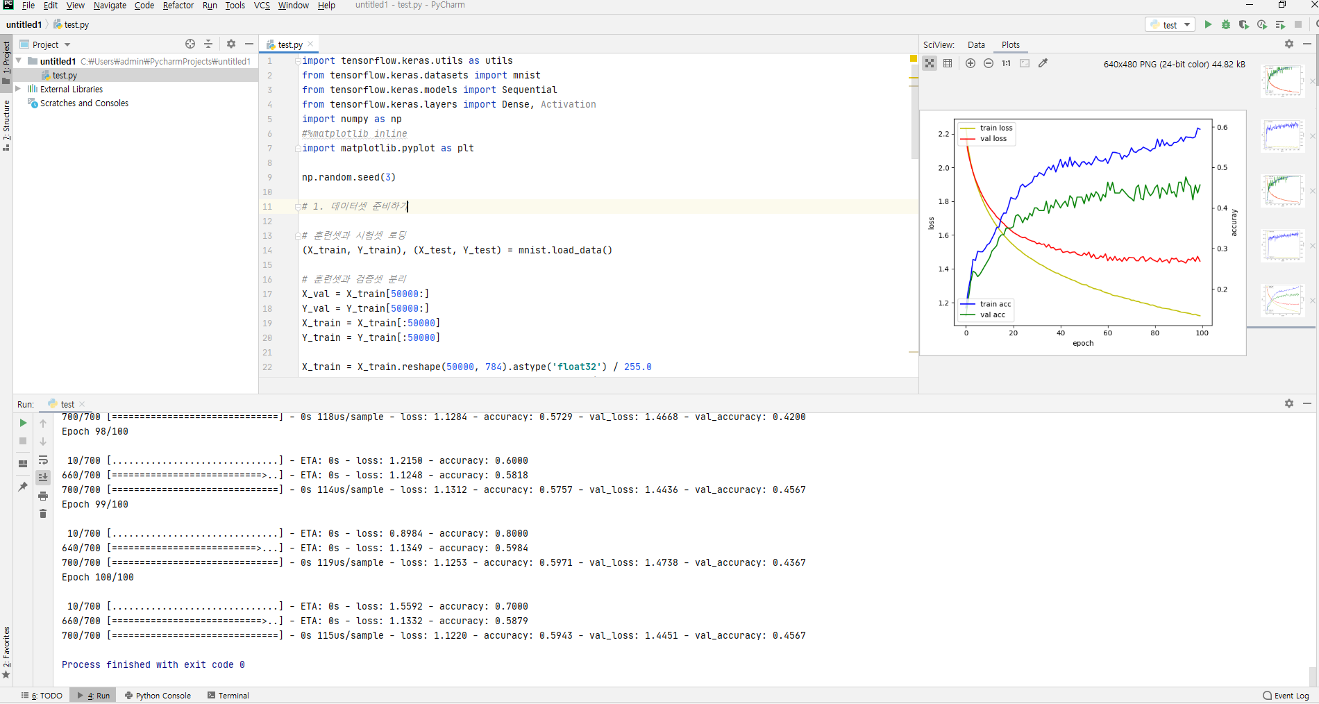

import tensorflow.keras.utils as utils
from tensorflow.keras.datasets import mnist
from tensorflow.keras.models import Sequential
from tensorflow.keras.layers import Dense, Activation
import numpy as np
#%matplotlib inline
import matplotlib.pyplot as plt

np.random.seed(3)

1. 데이터셋 준비하기

훈련셋과 시험셋 로딩

(X_train, Y_train), (X_test, Y_test) = mnist.load_data()

훈련셋과 검증셋 분리

X_val = X_train[50000:]
Y_val = Y_train[50000:]
X_train = X_train[:50000]
Y_train = Y_train[:50000]

X_train = X_train.reshape(50000, 784).astype('float32') / 255.0
X_val = X_val.reshape(10000, 784).astype('float32') / 255.0
X_test = X_test.reshape(10000, 784).astype('float32') / 255.0

훈련셋, 검증셋 고르기

train_rand_idxs = np.random.choice(50000, 700)
val_rand_idxs = np.random.choice(10000, 300)

X_train = X_train[train_rand_idxs]
Y_train = Y_train[train_rand_idxs]
X_val = X_val[val_rand_idxs]
Y_val = Y_val[val_rand_idxs]

라벨링 전환

Y_train = utils.to_categorical(Y_train)
Y_val = utils.to_categorical(Y_val)
Y_test = utils.to_categorical(Y_test)

2. 모델 구성하기

model = Sequential()
model.add(Dense(units=2, input_dim=28*28, activation='relu'))
model.add(Dense(units=10, activation='softmax'))

3. 모델 엮기

model.compile(loss='categorical_crossentropy', optimizer='sgd', metrics=['accuracy'])

4. 모델 학습시키기

hist = model.fit(X_train, Y_train, epochs=100, batch_size=10, validation_data=(X_val, Y_val))

fig, loss_ax = plt.subplots()

acc_ax = loss_ax.twinx()

loss_ax.plot(hist.history['loss'], 'y', label='train loss')
loss_ax.plot(hist.history['val_loss'], 'r', label='val loss')

acc_ax.plot(hist.history['accuracy'], 'b', label='train acc')
acc_ax.plot(hist.history['val_accuracy'], 'g', label='val acc')

loss_ax.set_xlabel('epoch')
loss_ax.set_ylabel('loss')
acc_ax.set_ylabel('accuray')

loss_ax.legend(loc='upper left')
acc_ax.legend(loc='lower left')

plt.show()

산 내려오는 작은 오솔길 잘찾기의 발달 계보

import tensorflow.keras.utils as utils
from tensorflow.keras.datasets import mnist
from tensorflow.keras.models import Sequential
from tensorflow.keras.layers import Dense, Activation
import numpy as np
#%matplotlib inline
import matplotlib.pyplot as plt
from numpy import argmax

np.random.seed(3)

1. 데이터셋 준비하기

훈련셋과 시험셋 로딩

(X_train, Y_train), (X_test, Y_test) = mnist.load_data()

훈련셋과 검증셋 분리

X_val = X_train[50000:]
Y_val = Y_train[50000:]
X_train = X_train[:50000]
Y_train = Y_train[:50000]

X_train = X_train.reshape(50000, 784).astype('float32') / 255.0
X_val = X_val.reshape(10000, 784).astype('float32') / 255.0
X_test = X_test.reshape(10000, 784).astype('float32') / 255.0

훈련셋, 검증셋 고르기

# train_rand_idxs = np.random.choice(50000, 700)
# val_rand_idxs = np.random.choice(10000, 300)
#
# X_train = X_train[train_rand_idxs]
# Y_train = Y_train[train_rand_idxs]
# X_val = X_val[val_rand_idxs]
# Y_val = Y_val[val_rand_idxs]

훈련셋과 검증셋 분리

x_val = X_val[:42000] # 훈련셋의 30%를 검증셋으로 사용
x_train = Y_val[42000:]
y_val = Y_train[:42000] # 훈련셋의 30%를 검증셋으로 사용
y_train = Y_train[42000:]

라벨링 전환

Y_train = utils.to_categorical(Y_train)
Y_val = utils.to_categorical(Y_val)
Y_test = utils.to_categorical(Y_test)

2. 모델 구성하기

model = Sequential()
model.add(Dense(units=64, input_dim=28*28, activation='relu'))
model.add(Dense(units=10, activation='softmax'))

3. 모델 엮기

model.compile(loss='categorical_crossentropy', optimizer='sgd', metrics=['accuracy'])

4. 모델 학습시키기

hist = model.fit(X_train, Y_train, epochs=5, batch_size=32, validation_data=(X_val, Y_val))

fig, loss_ax = plt.subplots()

acc_ax = loss_ax.twinx()

loss_ax.plot(hist.history['loss'], 'y', label='train loss')
loss_ax.plot(hist.history['val_loss'], 'r', label='val loss')

acc_ax.plot(hist.history['accuracy'], 'b', label='train acc')
acc_ax.plot(hist.history['val_accuracy'], 'g', label='val acc')

loss_ax.set_xlabel('epoch')
loss_ax.set_ylabel('loss')
acc_ax.set_ylabel('accuray')

loss_ax.legend(loc='upper left')
acc_ax.legend(loc='lower left')

plt.show()

5. 모델 평가하기

loss_and_metrics = model.evaluate(X_test, Y_test, batch_size=32)
print('')
print('loss_and_metrics : ' + str(loss_and_metrics))

6. 모델 사용하기

xhat_idx = np.random.choice(X_test.shape[0], 5)
xhat = X_test[xhat_idx]
yhat = model.predict_classes(xhat)

for i in range(5):
print('True : ' + str(argmax(Y_test[xhat_idx[i]])) + ', Predict : ' + str(yhat[i]))

피마족 인디언 당뇨병 발병 데이터셋

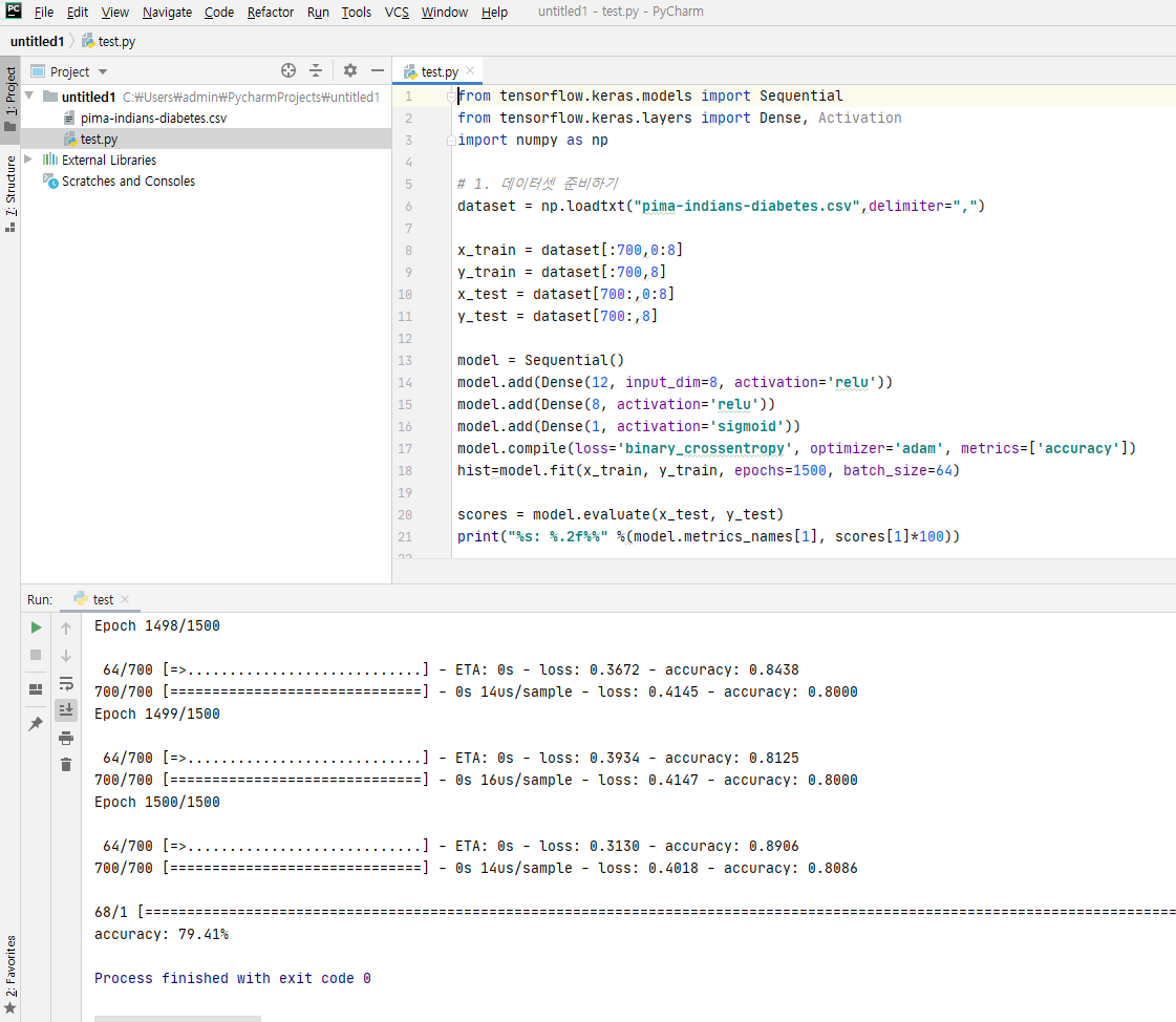
from tensorflow.keras.models import Sequential
from tensorflow.keras.layers import Dense, Activation
import numpy as np

1. 데이터셋 준비하기

dataset = np.loadtxt("pima-indians-diabetes.csv",delimiter=",")

x_train = dataset[:700,0:8]
y_train = dataset[:700,8]
x_test = dataset[700:,0:8]
y_test = dataset[700:,8]

model = Sequential()
model.add(Dense(12, input_dim=8, activation='relu'))
model.add(Dense(8, activation='relu'))
model.add(Dense(1, activation='sigmoid'))
model.compile(loss='binary_crossentropy', optimizer='adam', metrics=['accuracy'])
hist=model.fit(x_train, y_train, epochs=1500, batch_size=64)

scores = model.evaluate(x_test, y_test)
print("%s: %.2f%%" %(model.metrics_names[1], scores[1]*100))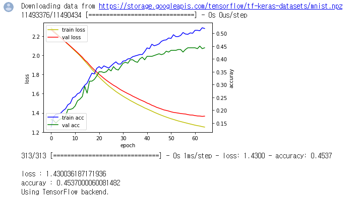

import tensorflow as tf
import tensorflow.keras.utils as utils
from tensorflow.keras.datasets import mnist
from tensorflow.keras.models import Sequential
from tensorflow.keras.layers import Dense, Activation
import numpy as np
import matplotlib.pyplot as plt
#%matplotlib inline

np.random.seed(3)

1. 데이터셋 준비하기

훈련셋과 시험셋 로딩

(X_train, Y_train), (X_test, Y_test) = mnist.load_data()

# 훈련셋과 검증셋 분리
X_val = X_train[50000:]
Y_val = Y_train[50000:]
X_train = X_train[:50000]
Y_train = Y_train[:50000]

X_train = X_train.reshape(50000, 784).astype('float32') / 255.0
X_val = X_val.reshape(10000, 784).astype('float32') / 255.0
X_test = X_test.reshape(10000, 784).astype('float32') / 255.0

훈련셋, 검증셋 고르기

train_rand_idxs = np.random.choice(50000, 700)
val_rand_idxs = np.random.choice(10000, 300)

X_train = X_train[train_rand_idxs]
Y_train = Y_train[train_rand_idxs]
X_val = X_val[val_rand_idxs]
Y_val = Y_val[val_rand_idxs]

라벨링 전환

Y_train = utils.to_categorical(Y_train)
Y_val = utils.to_categorical(Y_val)
Y_test = utils.to_categorical(Y_test)

2. 모델 구성하기

model = Sequential()
model.add(Dense(units=2, input_dim=28*28, activation='relu'))
model.add(Dense(units=10, activation='softmax'))

3. 모델 엮기

model.compile(loss='categorical_crossentropy', optimizer='sgd', metrics=['accuracy'])

4. 모델 학습시키기

from tensorflow.keras.callbacks import EarlyStopping
early_stopping = EarlyStopping() # 조기종료 콜백함수 정의
hist = model.fit(X_train, Y_train, epochs=1000, batch_size=10, verbose=0, validation_data=(X_val, Y_val), callbacks=[early_stopping])

fig, loss_ax = plt.subplots()

acc_ax = loss_ax.twinx()

loss_ax.plot(hist.history['loss'], 'y', label='train loss')
loss_ax.plot(hist.history['val_loss'], 'r', label='val loss')

acc_ax.plot(hist.history['accuracy'], 'b', label='train acc')
acc_ax.plot(hist.history['val_accuracy'], 'g', label='val acc')

loss_ax.set_xlabel('epoch')
loss_ax.set_ylabel('loss')
acc_ax.set_ylabel('accuray')

loss_ax.legend(loc='upper left')
acc_ax.legend(loc='lower left')

plt.show()

6. 모델 사용하기

loss_and_metrics = model.evaluate(X_test, Y_test, batch_size=32)

print('')
print('loss : ' + str(loss_and_metrics[0]))
print('accuray : ' + str(loss_and_metrics[1]))

6. 모델 저장하기

from tensorflow.keras.models import load_model
model.save('mnist_mlp_model.h5')

1. 실무에 사용할 데이터 준비하기

(x_train, y_train), (x_test, y_test) = mnist.load_data()
x_test = x_test.reshape(10000, 784).astype('float32') / 255.0
y_test = utils.to_categorical(y_test)
xhat_idx = np.random.choice(x_test.shape[0], 5)
xhat = x_test[xhat_idx]

2. 모델 불러오기

from tensorflow.keras.models import load_model
model = load_model('mnist_mlp_model.h5')

3. 모델 사용하기

yhat = model.predict_classes(xhat)

for i in range(5):
print('True : ' + str(np.argmax(y_test[xhat_idx[i]])) + ', Predict : ' + str(yhat[i]))

콜백함수

import tensorflow as tf
import tensorflow.keras.utils as utils
from tensorflow.keras.datasets import mnist
from tensorflow.keras.models import Sequential
from tensorflow.keras.layers import Dense, Activation
import numpy as np
import matplotlib.pyplot as plt
# %matplotlib inline

class CustomHistory(tf.keras.callbacks.Callback):
def init(self):
self.epoch = 0
self.train_loss = []
self.val_loss = []
self.train_acc = []
self.val_acc = []

def on_epoch_end(self, batch, logs={}):
self.train_loss.append(logs.get('loss'))
self.val_loss.append(logs.get('val_loss'))
self.train_acc.append(logs.get('acc'))
self.val_acc.append(logs.get('val_acc'))
if self.epoch % 100 == 0:
print("epoch: {0} - loss: {1:8.6f}".format(self.epoch, logs.get('loss')))

self.epoch += 1

(X_train, Y_train), (X_test, Y_test) = mnist.load_data()

훈련셋과 검증셋 분리

X_val = X_train[50000:]
Y_val = Y_train[50000:]
X_train = X_train[:50000]
Y_train = Y_train[:50000]

X_train = X_train.reshape(50000, 784).astype('float32') / 255.0
X_val = X_val.reshape(10000, 784).astype('float32') / 255.0
X_test = X_test.reshape(10000, 784).astype('float32') / 255.0

훈련셋, 검증셋 고르기

train_rand_idxs = np.random.choice(50000, 700)
val_rand_idxs = np.random.choice(10000, 300)

X_train = X_train[train_rand_idxs]
Y_train = Y_train[train_rand_idxs]
X_val = X_val[val_rand_idxs]
Y_val = Y_val[val_rand_idxs]

라벨링 전환

Y_train = utils.to_categorical(Y_train)
Y_val = utils.to_categorical(Y_val)
Y_test = utils.to_categorical(Y_test)

2. 모델 구성하기

model = Sequential()
model.add(Dense(units=2, input_dim=28 * 28, activation='relu'))
model.add(Dense(units=10, activation='softmax'))

3. 모델 엮기

model.compile(loss='categorical_crossentropy', optimizer='sgd', metrics=['accuracy'])

4. 모델 학습시키기

custom_hist = CustomHistory()
custom_hist.init()

for epoch_idx in range(1000):
# print ('epochs : ' + str(epoch_idx) )
model.fit(X_train, Y_train, epochs=1, batch_size=10, verbose=0, validation_data=(X_val, Y_val),
callbacks=[custom_hist])

fig, loss_ax = plt.subplots()

acc_ax = loss_ax.twinx()

loss_ax.plot(custom_hist.train_loss, 'y', label='train loss')
loss_ax.plot(custom_hist.val_loss, 'r', label='val loss')


loss_ax.set_xlabel('epoch')
loss_ax.set_ylabel('loss')

loss_ax.legend(loc='upper left')

plt.show()

6. 모델 사용하기

loss_and_metrics = model.evaluate(X_test, Y_test, batch_size=32)

print('')
print('loss : ' + str(loss_and_metrics[0]))
print('accuray : ' + str(loss_and_metrics[1]))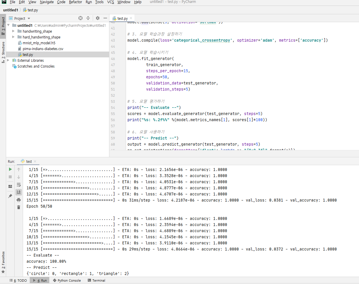

pip install pillow 
pip install SciPy

import numpy as np
from tensorflow.keras.models import Sequential
from tensorflow.keras.layers import Dense
from tensorflow.keras.layers import Flatten
from tensorflow.keras.layers import Conv2D
from tensorflow.keras.layers import MaxPooling2D
from tensorflow.keras.preprocessing.image import ImageDataGenerator

랜덤시드 고정시키기

np.random.seed(3)

1. 데이터 생성하기

train_datagen = ImageDataGenerator(rescale=1./255)

train_generator = train_datagen.flow_from_directory(
'handwriting_shape/train',
target_size=(24, 24),
batch_size=3,
class_mode='categorical')

test_datagen = ImageDataGenerator(rescale=1./255)

test_generator = test_datagen.flow_from_directory(
'handwriting_shape/test',
target_size=(24, 24),
batch_size=3,
class_mode='categorical')

2. 모델 구성하기

model = Sequential()
model.add(Conv2D(32, kernel_size=(3, 3),
activation='relu',
input_shape=(24,24,3)))
model.add(Conv2D(64, (3, 3), activation='relu'))
model.add(MaxPooling2D(pool_size=(2, 2)))
model.add(Flatten())
model.add(Dense(128, activation='relu'))
model.add(Dense(3, activation='softmax'))

3. 모델 학습과정 설정하기

model.compile(loss='categorical_crossentropy', optimizer='adam', metrics=['accuracy'])

4. 모델 학습시키기

model.fit_generator(
train_generator,
steps_per_epoch=15,
epochs=50,
validation_data=test_generator,
validation_steps=5)

5. 모델 평가하기

print("-- Evaluate --")
scores = model.evaluate_generator(test_generator, steps=5)
print("%s: %.2f%%" %(model.metrics_names[1], scores[1]*100))

6. 모델 사용하기

print("-- Predict --")
output = model.predict_generator(test_generator, steps=5)
np.set_printoptions(formatter={'float': lambda x: "{0:0.3f}".format(x)})
print(test_generator.class_indices)
print(output)

컨볼루션 신경망 레이어

문제 정의하기

문제 형태: 다중 클래스 분류
입력: 손으로 그린 삼각형, 사각형, 원 이미지
출력: 삼각형, 사각형, 원일 확률을 나타내는 벡터

Dropout - 앙상블효과로 성능이 향상 됨

!pip install tensorflow-gpu

import tensorflow as tf
import numpy as np
from tensorflow.keras import datasets, layers, models
from matplotlib import pyplot as plt
from tensorflow.keras import layers
from tensorflow.keras import Input
from tensorflow.keras import Model

import tensorflow as tf
import numpy as np
from tensorflow.keras.models import Sequential
from tensorflow.keras.layers import Dense
from tensorflow.keras.layers import Flatten
from tensorflow.keras.layers import Conv2D
from tensorflow.keras.layers import MaxPooling2D
from tensorflow.keras.layers import Dropout

keras 데이터 가져오기

cifar10_data = tf.keras.datasets.cifar10.load_data()
((train_data, train_label), (test_data, test_label)) = cifar10_data

print("train_data_num: {0}, \ntest_data_num: {1}, \ntrain_label_num: {2}, \ntest_label_num: {3},".format(len(train_data), len(test_data), len(train_label), len(test_label)))

import tensorflow as tf

print(tf.__version__)
import tensorflow.keras.utils as utils
import numpy as np
from tensorflow.keras.datasets import mnist
from tensorflow.keras.models import Sequential
from tensorflow.keras.layers import Dense, Activation
from tensorflow.keras.layers import Conv2D, MaxPooling2D, Flatten
from tensorflow.keras.layers import Dropout

width = 28
height = 28

1. 데이터셋 생성하기

훈련셋과 시험셋 불러오기

(x_train, y_train), (x_test, y_test) = mnist.load_data()
x_train = x_train.reshape(60000, width, height, 1).astype('float32') / 255.0
x_test = x_test.reshape(10000, width, height, 1).astype('float32') / 255.0

훈련셋과 검증셋 분리

x_val = x_train[50000:]
y_val = y_train[50000:]
x_train = x_train[:50000]
y_train = y_train[:50000]

데이터셋 전처리 : one-hot 인코딩

y_train = utils.to_categorical(y_train)
y_val = utils.to_categorical(y_val)
y_test = utils.to_categorical(y_test)

2. 모델 구성하기

model = Sequential()
model.add(Conv2D(32, (3, 3), activation='relu', input_shape=(width, height, 1)))
model.add(Conv2D(32, (3, 3), activation='relu'))
model.add(MaxPooling2D(pool_size=(2, 2)))
model.add(Dropout(0.25))
model.add(Conv2D(64, (3, 3), activation='relu'))
model.add(Conv2D(64, (3, 3), activation='relu'))
model.add(MaxPooling2D(pool_size=(2, 2)))
model.add(Dropout(0.25))
model.add(Flatten())
model.add(Dense(256, activation='relu'))
model.add(Dropout(0.5))
model.add(Dense(10, activation='softmax'))

3. 모델 학습과정 설정하기

model.compile(loss='categorical_crossentropy', optimizer='sgd', metrics=['accuracy'])

4. 모델 학습시키기

hist = model.fit(x_train, y_train, epochs=30, batch_size=32, validation_data=(x_val, y_val))

5. 학습과정 살펴보기

# % matplotlib
# inline
import matplotlib.pyplot as plt

fig, loss_ax = plt.subplots()

acc_ax = loss_ax.twinx()

loss_ax.plot(hist.history['loss'], 'y', label='train loss')
loss_ax.plot(hist.history['val_loss'], 'r', label='val loss')
loss_ax.set_ylim([0.0, 0.5])

acc_ax.plot(hist.history['accuracy'], 'b', label='train acc')
acc_ax.plot(hist.history['val_accuracy'], 'g', label='val acc')
acc_ax.set_ylim([0.8, 1.0])

loss_ax.set_xlabel('epoch')
loss_ax.set_ylabel('loss')
acc_ax.set_ylabel('accuray')

loss_ax.legend(loc='upper left')
acc_ax.legend(loc='lower left')

plt.show()

6. 모델 평가하기

loss_and_metrics = model.evaluate(x_test, y_test, batch_size=32)
print('## evaluation loss and_metrics ##')
print(loss_and_metrics)

7. 모델 사용하기

yhat_test = model.predict(x_test, batch_size=32)

# % matplotlib
# inline
import matplotlib.pyplot as plt

plt_row = 5
plt_col = 5

plt.rcParams["figure.figsize"] = (10, 10)

f, axarr = plt.subplots(plt_row, plt_col)

cnt = 0
i = 0

while cnt < (plt_row * plt_col):

if np.argmax(y_test[i]) == np.argmax(yhat_test[i]):
i += 1
continue

sub_plt = axarr[int(cnt / plt_row), int(cnt % plt_col)]
sub_plt.axis('off')
sub_plt.imshow(x_test[i].reshape(width, height))
sub_plt_title = 'R: ' + str(np.argmax(y_test[i])) + ' P: ' + str(np.argmax(yhat_test[i]))
sub_plt.set_title(sub_plt_title)

i += 1
cnt += 1

plt.show()

print(tf.__version__)
import tensorflow.keras.utils as utils
from tensorflow.keras.datasets import mnist
from tensorflow.keras.models import Sequential
from tensorflow.keras.layers import Dense, Activation
import numpy as np

width = 28
height = 28

1. 데이터셋 생성하기

훈련셋과 시험셋 불러오기

(x_train, y_train), (x_test, y_test) = mnist.load_data()
x_train = x_train.reshape(60000, width * height).astype('float32') / 255.0
x_test = x_test.reshape(10000, width * height).astype('float32') / 255.0

훈련셋과 검증셋 분리

x_val = x_train[50000:]
y_val = y_train[50000:]
x_train = x_train[:50000]
y_train = y_train[:50000]

데이터셋 전처리 : one-hot 인코딩

y_train = utils.to_categorical(y_train)
y_val = utils.to_categorical(y_val)
y_test = utils.to_categorical(y_test)

2. 모델 구성하기

model = Sequential()
model.add(Dense(256, input_dim=width * height, activation='relu'))
model.add(Dense(256, activation='relu'))
model.add(Dense(256, activation='relu'))
model.add(Dense(256, activation='relu'))
model.add(Dense(10, activation='softmax'))

3. 모델 학습과정 설정하기

model.compile(loss='categorical_crossentropy', optimizer='sgd', metrics=['accuracy'])

4. 모델 학습시키기

hist = model.fit(x_train, y_train, epochs=50, batch_size=32, validation_data=(x_val, y_val))

5. 학습과정 살펴보기

# % matplotlib
# inline
import matplotlib.pyplot as plt

fig, loss_ax = plt.subplots()

acc_ax = loss_ax.twinx()

loss_ax.plot(hist.history['loss'], 'y', label='train loss')
loss_ax.plot(hist.history['val_loss'], 'r', label='val loss')
loss_ax.set_ylim([0.0, 0.5])

acc_ax.plot(hist.history['accuracy'], 'b', label='train acc')
acc_ax.plot(hist.history['val_accuracy'], 'g', label='val acc')
acc_ax.set_ylim([0.8, 1.0])

loss_ax.set_xlabel('epoch')
loss_ax.set_ylabel('loss')
acc_ax.set_ylabel('accuray')

loss_ax.legend(loc='upper left')
acc_ax.legend(loc='lower left')

plt.show()

6. 모델 평가하기

loss_and_metrics = model.evaluate(x_test, y_test, batch_size=32)
print('## evaluation loss and_metrics ##')
print(loss_and_metrics)

7. 모델 사용하기

yhat_test = model.predict(x_test, batch_size=32)

# % matplotlib
# inline
import matplotlib.pyplot as plt

plt_row = 5
plt_col = 5

plt.rcParams["figure.figsize"] = (10, 10)

f, axarr = plt.subplots(plt_row, plt_col)

cnt = 0
i = 0

while cnt < (plt_row * plt_col):

if np.argmax(y_test[i]) == np.argmax(yhat_test[i]):
i += 1
continue

sub_plt = axarr[int(cnt / plt_row), int(cnt % plt_col)]
sub_plt.axis('off')
sub_plt.imshow(x_test[i].reshape(width, height))
sub_plt_title = 'R: ' + str(np.argmax(y_test[i])) + ' P: ' + str(np.argmax(yhat_test[i]))
sub_plt.set_title(sub_plt_title)

i += 1
cnt += 1

plt.show()

import tensorflow as tf

print(tf.__version__)

import numpy as np
from tensorflow.keras.models import Sequential
from tensorflow.keras.layers import Dense, LSTM
import tensorflow.keras.utils as utils
import os

# http://web.mit.edu/music21/doc/usersGuide/usersGuide_08_installingMusicXML.html
import music21

seq = ['g8', 'e8', 'e4', 'f8', 'd8', 'd4', 'c8', 'd8', 'e8', 'f8', 'g8', 'g8', 'g4',
'g8', 'e8', 'e8', 'e8', 'f8', 'd8', 'd4', 'c8', 'e8', 'g8', 'g8', 'e8', 'e8', 'e4',
'd8', 'd8', 'd8', 'd8', 'd8', 'e8', 'f4', 'e8', 'e8', 'e8', 'e8', 'e8', 'f8', 'g4',
'g8', 'e8', 'e4', 'f8', 'd8', 'd4', 'c8', 'e8', 'g8', 'g8', 'e8', 'e8', 'e4']

print("length of seq: {0}".format(len(seq)))

note_seq = ""
for note in seq:
note_seq += note + " "

m = music21.converter.parse("2/4 " + note_seq, format='tinyNotation')

m.show("midi")

m.show()

code2idx = {'c4': 0, 'd4': 1, 'e4': 2, 'f4': 3, 'g4': 4, 'a4': 5, 'b4': 6,
'c8': 7, 'd8': 8, 'e8': 9, 'f8': 10, 'g8': 11, 'a8': 12, 'b8': 13}

idx2code = {0: 'c4', 1: 'd4', 2: 'e4', 3: 'f4', 4: 'g4', 5: 'a4', 6: 'b4',
7: 'c8', 8: 'd8', 9: 'e8', 10: 'f8', 11: 'g8', 12: 'a8', 13: 'b8'}


def seq2dataset(seq, window_size):
dataset = []

for i in range(len(seq) - window_size):
subset = seq[i: (i + window_size + 1)]
dataset.append([code2idx[item] for item in subset])
return np.array(dataset)


test_seq = ['c4', 'd4', 'e4', 'f4', 'g4', 'd8', 'b8']
dataset = seq2dataset(seq=test_seq, window_size=4)
print(dataset)

n_steps = 4
n_inputs = 1

dataset = seq2dataset(seq, window_size=n_steps)

print("dataset.shape: {0}".format(dataset.shape))

x_train = dataset[:, 0: n_steps]
y_train = dataset[:, n_steps]
print("x_train: {0}".format(x_train.shape))
print("y_train: {0}".format(y_train.shape))
print(x_train[0])
print(y_train[0])

max_idx_value = len(code2idx) - 1

print("max_idx_value: {0}".format(max_idx_value))

x_train = x_train / float(max_idx_value)

x_train = np.reshape(x_train, (x_train.shape[0], x_train.shape[1], n_inputs))

y_train = utils.to_categorical(y_train)

one_hot_vec_size = y_train.shape[1]

print("one hot encoding vector size is {0}".format(one_hot_vec_size))
print("After pre-processing")
print("x_train: {0}".format(x_train.shape))
print("y_train: {0}".format(y_train.shape))

model = Sequential()
model.add(LSTM(
units=128,
kernel_initializer='glorot_normal',
bias_initializer='zero',
batch_input_shape=(1, n_steps, n_inputs),
stateful=True
))
model.add(Dense(
units=one_hot_vec_size,
kernel_initializer='glorot_normal',
bias_initializer='zero',
activation='softmax'
))

model.compile(
loss='categorical_crossentropy',
optimizer='adam',
metrics=['accuracy']
)


class LossHistory(tf.keras.callbacks.Callback):
def init(self):
self.epoch = 0
self.losses = []

def on_epoch_end(self, batch, logs={}):
self.losses.append(logs.get('loss'))

if self.epoch % 100 == 0:
print("epoch: {0} - loss: {1:8.6f}".format(self.epoch, logs.get('loss')))

self.epoch += 1


num_epochs = 1500
history = LossHistory() # 손실 이력 객체 생성

history.init()

for epoch_idx in range(num_epochs + 1):
model.fit(
x=x_train,
y=y_train,
epochs=1,
batch_size=1,
verbose=0,
shuffle=False,
callbacks=[history]
)
if history.losses[-1] < 1e-5:
print("epoch: {0} - loss: {1:8.6f}".format(epoch_idx, history.losses[-1]))
model.reset_states()
break
model.reset_states()

import matplotlib.pyplot as plt
% matplotlib
inline

plt.plot(history.losses)
plt.ylabel('loss')
plt.xlabel('epoch')
plt.legend(['train'], loc='upper right')
plt.show()

scores = model.evaluate(x_train, y_train, batch_size=1)
print("{0}: {1}".format(model.metrics_names[1], scores[1] * 100))
model.reset_states()

pred_count = 50 # 최대 예측 개수 정의

한 스텝 예측

seq_out = ['g8', 'e8', 'e4', 'f8']
pred_out = model.predict(x_train)

for i in range(pred_count):
idx = np.argmax(pred_out[i]) # one-hot 인코딩을 인덱스 값으로 변환
seq_out.append(idx2code[idx]) # seq_out는 최종 악보이므로 인덱스 값을 코드로 변환하여 저장

model.reset_states()

print("one step prediction : ", seq_out)

seq_in = ['g8', 'c8', 'f4', 'e8']
seq_out = seq_in
seq_in = [code2idx[note] / float(max_idx_value) for note in seq_in] # 코드를 인덱스값으로 변환

for i in range(pred_count):
sample_in = np.array(seq_in)
sample_in = np.reshape(sample_in, (1, n_steps, n_inputs)) # 샘플 수, 타입스텝 수, 속성 수
pred_out = model.predict(sample_in)
idx = np.argmax(pred_out)
seq_out.append(idx2code[idx])
seq_in.append(idx / float(max_idx_value))
seq_in.pop(0)

model.reset_states()

print("full song prediction : ")

for note in seq_out:
print(note, end=" ")

# http://web.mit.edu/music21/doc/usersGuide/usersGuide_08_installingMusicXML.html
import music21

note_seq = ""
for note in seq_out:
note_seq += note + " "

conv_midi = music21.converter.subConverters.ConverterMidi()

m = music21.converter.parse("2/4 " + note_seq, format='tinyNotation')

m.show("midi")

m.show()

m.write("midi", fp="./new_music.mid")

김경민

이전 포스트

딥러닝을 활용한 자연어 처리

다음 포스트