https://www.youtube.com/watch?v=CS4cs9xVecg&list=PLkDaE6sCZn6Ec-XTbcX1uRg2_u4xOEky0

Andrew Ng 의 Machine Learning Course 01의 Week 1 ~ Week 2 를 수강하고 정리하였습니다.

Introduction

What is a Neural Network?

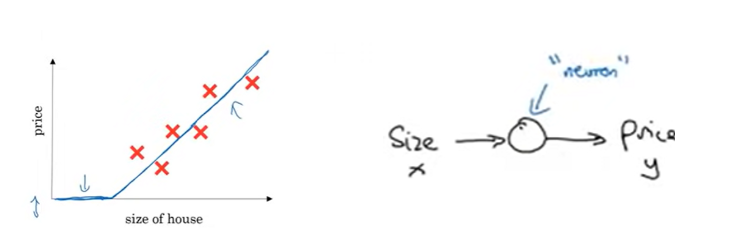
Housing Price Prediction example

Tiny neural network:

By stacking many neurons, you can get a bigger neural network:

X는 input layer, y는 output layer, X, y 사이의 neurons는 hidden layer이다.

Supervised Learning with a Neural Network

supervised learning needs input X and output y:

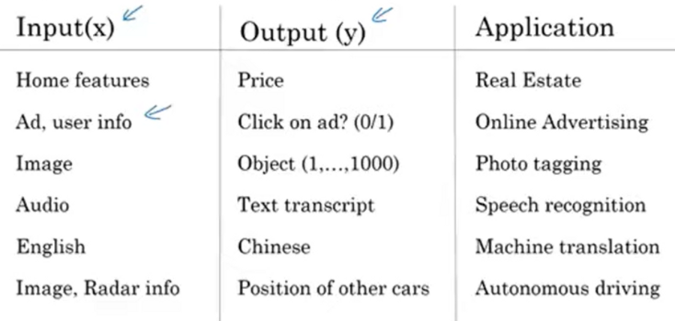
→ selecting X and y is important

• Real Estate and Online Advertising uses standard neural network
• Photo taggin uses CNN
• Speech Recognition and Machine translation uses RNN (1-d sequence data에 RNN 잘 사용)
• Autonomous driving uses Custom/Hybrid architecture (input으로 Image, Radar 등 다양한 정보가 들어가므로)

Neural Network examples

Structured data and unstructured data

rise of neural network → computers can understand unstructured data much better!

Why is deep learning taking off?

Scale drives deep learning progress

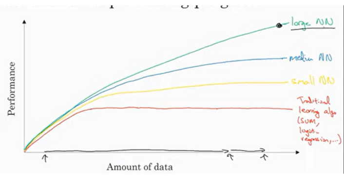
• Traditional learning algorithms as SVM, performance improves when amount of data increases but at some point it flattens.
• last 20 years, amount of data has rapidly increased!
• As for Neural Network, the larger the neural network, the performance increases more as amount of data gets larger.

m: number of training examples (size of training data)

⇒ Scale of data (m) drives deep learning progress!

• data (m)
• computation
• algorithms

using sigmoid function → 그래프 양 끝의 gradient가 0에 가까워 learning 속도가 매우 느려진다. (parameter가 천천히 바뀌기 때문)

ReLU 사용 → sigmoid를 사용했을 때보다gradient descent가 훨씬 빨라졌다

Basics of Neural Network programming

forward propagation and backward propagation

Binary Classification

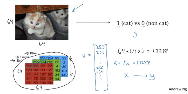
pixel intensity values → input feature vector x 로 바꾸려면 먼저 featue vector x 를 define 해야 한다.

Notation

• x is n_x dimensional feature vector
• y is 0 or 1
• m training examples

define a matrix X and stack m training examples as columns

• n_x rows
• m columns
• X.shape = (n_x, m)

define Y matrix

• Y.shape = (1, m)

Logistic Regression

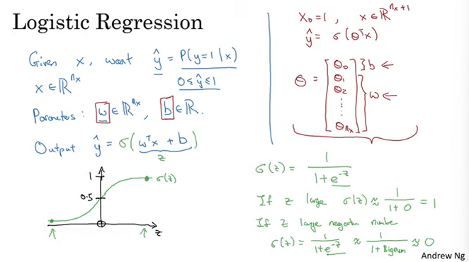
Given input feature vector x, want y^ to be P(y=1|x), which means the chance of the given x to be a cat picture.

with given x and parameters are w and b, how do we generage output y^?

• y^ = $w^Tx + b$ 와 같은 식을 사용해 구할 수 있지만, y^이 0~1 의 값을 가지게 하고 싶다면
• y^ = $sigmoid(w^Tx + b)$ 처럼 sigmoid 를 사용해야 한다.

Logistic Regression cost function

model output인 y^ 와 ground truth인 y 를 비교해 loss 계산

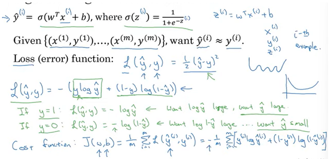
terminoloogy:

• Loss function is applied to just single training example
• cost function is the cost of your parameters (w, b)

Gradient Descent

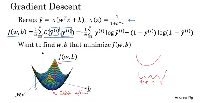
parameter w, b에 따른 cost function J(w, b)

⇒ J(w, b) 가 minimum인 w, b를 찾는 것이 목적이다.

one local minima → convex function
many local minima → nonconvex function

gradient descent : from initialized value, step downhill and find minima!

: actual update of w and b

derivative를 뜻하는 d는 partial derivative를 뜻하는 다른 기호로 나타내지기도 한다.

Derivatives

derivative = slope = height/width

at a = 2, slope is 3

at a = 5, slope is also 3

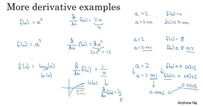
More Derivatives Examples

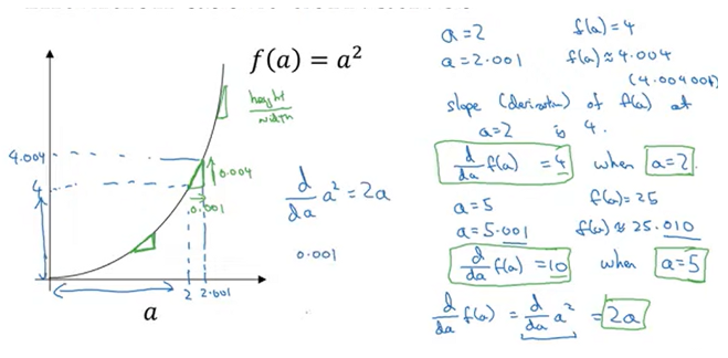
at a = 2, slope is 4

at a = 5, slope is 10

derivative of a^2 is 2a (Calculus)

Computation Graph

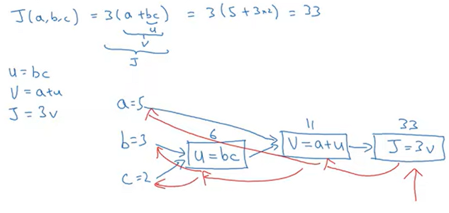
• computing J(a, b, c) needs three steps: u, v, J
• blue arrow : forward pass
• red arrow : backward pass

Computing derivatives

if you change a, value of v changes and therefore changes J.

dJ/da 를 구하기 위해서는 dJ/dv 와 dv/da 를 먼저 구해야 한다 ⇒ backward propagation

• final output variable is J in this graph.
• you want to calculate dJ/dvar

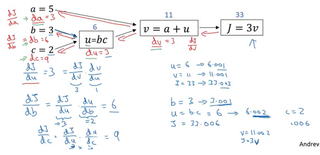
dJ/du is dJ/dv * dv/du

using chain rule, dJ/db = dJ/du * du/db

dJ/dc = dJ/du * du/dc

⇒ to compue all the derivatives, most effecient way is to compute from right to left. (backward propagation)

Logistic Regression Gradient Descent

→ draw computational graph

→ modify w and b to reduce L(a, y) by going backward to compute derivatives

1. compute derivative da = dL/da = -y/a + (1-y)/(1-a)
2. compute derivative dz = dL/dz = dL/da * da/dz = a - y
3. dL/dw1 = x1 * dz
4. dL/dw2 = x2 * dz
5. db = dz

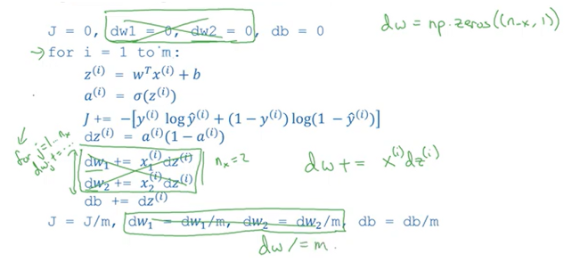
Gradient Descent on m Examples

Logistic regression on m examples

cost function J(w, b) is average of individual losses.

derivative of cost function J(w, b) is also average of derivatives of individual losses.

we are using dw_1, dw_2, db as accumulators.

after the algorithm, we can update parameters w_1, w_2, b.

for loops

• for i=1 to m
• for each features (dz, dw_1, dw_2, db, …)

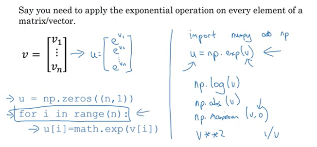
Vectorization can get rid of for loops → efficient!

Vectorization

What is vectorization?

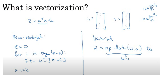
Non-vectorized implementations → for loops → very slow

vectorized → faster

demo

Google Colaboratory

More Vectorization Examples

Neural network programming guideline

Whenever possible, avoid explicit for-loops:

Vectors and matrix valued functions

Logistic regression derivatives

Vectorizing Logistic Regression

define X

and define Z

and define A

Vectorizing Logistic Regression’s Gradient Computation

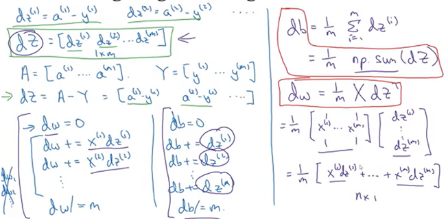
based on the definitions of dZ, we can compute this by one line of code!

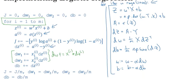
→ implementing logistic regression

Broadcasting in Python

Broadcasting example

• calculate percentage of callories from carb, protein, fat for each food.
  • carb in apples = 16/59 → 90%
• do this without for-loop! Google Colaboratory

  cal = A.sum(axis = 0)
  percentage = 100*A/(cal.reshape(1,4))
  		# you don't have to call reshape command.
  		# why? broadcasting

• (4, 1) + (1, ) ⇒ (4, 1) + (4, 1)
• (2, 3) + (1, 3) ⇒ (2, 3) + (2, 3)
• (m, n) + (m, 1) ⇒ (m, n) + (m, n)

General Principle

A Note on Python/Numpy Vectors

Google Colaboratory

illimate rank 1 array!!

Explanation of Logistic Regression’s Cost Function (Optional)

Logistic regression cost function

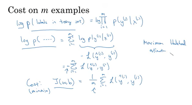
Cost on m examples