ADC
analog to digital converter
import numpy as np
import matplotlib.pyplot as plt
X_analog = np.linspace(0, 2*np.pi, 1000) #1초 음성 신호 가정
y_analog = np.sin(X_analog) * 10.0/2.0
X_digital = np.linspace(0, 2*np.pi, 10) # 디지털 샘플링(sampling rate : 60hz)
y_digital = (np.sin(X_digital) * 10.0/2.0).astype(int)
plt.plot(X_analog, y_analog)
plt.plot(X_digital,y_digital, "o")
plt.legend(["analog","digital_quantized"])
plt.show()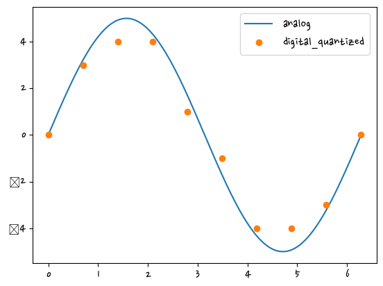
cd음질 44100hz, old전화기: 8000hz, 음성: 16000hz, 고급 192000hz
진폭 표현력 8bit, 16bit, 24bit
파형의 종류
sin, cos : 정현파, sinusoidal signal
임펄스(Impulse, 충격)
#impulse
X_analog = np.linspace(0, 2*np.pi, 1000)
y_analog = np.zeros(1000)
y_analog[500] = 1
plt.plot(X_analog, y_analog)
plt.show()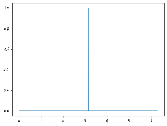
#unit function, 소리가 없다가 갑자기 생김
X_analog = np.linspace(0, 2*np.pi, 1000)
y_analog = np.zeros(1000)
y_analog[500:] = 1
plt.plot(X_analog, y_analog)
plt.show()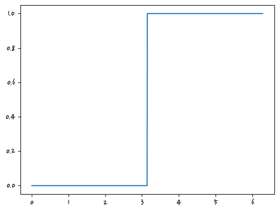
#exponential function
X_analog = np.linspace(0, 2*np.pi, 1000)
y_analog = np.ones(1000)
y_analog = y_analog * np.exp(X_analog)
#y_analog
plt.plot(X_analog, y_analog)
plt.show() 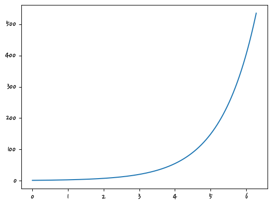
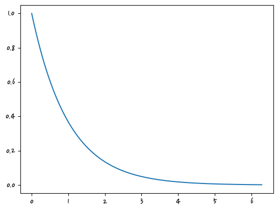
#exponential function
X_analog = np.linspace(0, 2*np.pi, 1000)
y_analog = np.ones(1000)
y_analog = y_analog * np.exp(-X_analog)
#y_analog
plt.plot(X_analog, y_analog)
plt.show()
X_digital = np.linspace(0, 2*np.pi, 50) # 디지털 샘플링(sampling rate : 60hz)
y_digital = np.sin(X_digital) #1초 1주기
y_digital2 = np.sin(X_digital*2) #1초 2주기
y_digital3 = np.sin(X_digital*3) #1초 3주기, 주파수 3hz 89.1mhz kbs fm 89100000hz, 악기튜닝할 때'라'음(440hz)으로 함


plt.plot(X_digital,y_digital, "o-")
plt.plot(X_digital,y_digital2, "o-")
plt.plot(X_digital,y_digital3, "o-")
plt.legend(["digital_0", "digital_2", "digital_3"])
plt.show()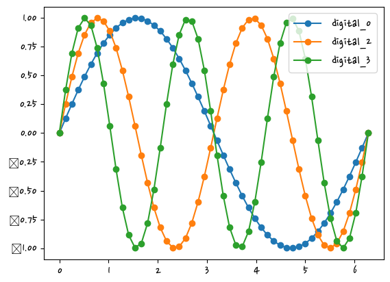
psycho-acoustics
w/ 우퍼220 - 12khz
w/o 우퍼440 - 12khz
220 440 880 1000 1500
440 900 1100 1600
220 440 880 1000 1500
진동수, 주파수 ,f(frequency), 단위 : hz
샘플링 주파수 fs
1초 신호, fs:8000 vs fs:16000
fs8000[0~7999]
fs16000[0~15999]
fs = 100 #샘플링 주파수
dt = 1/fs #샘플 간 시간
N = 300 #샘플 개수(3초)
t = np.arange(0, N) * dtsignal_1 = 1.0 * np.sin(2*np.pi * t)plt.figure(figsize=(8,2))
plt.plot(t, signal_1)
plt.title("1Hz 3 seconds")
plt.xlabel("second")
plt.ylabel("volume")
plt.show()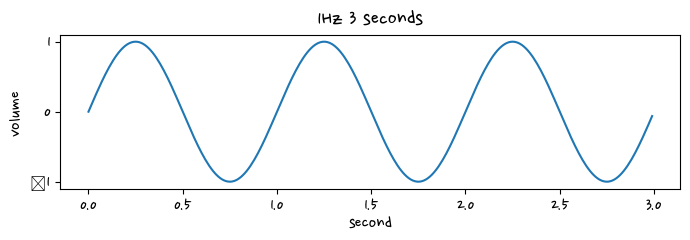
signal_2 = 0.3 * np.sin(2*np.pi * 3*t) # volume =0.3, 음높이 = 3*tplt.figure(figsize=(8,2))
plt.plot(t, signal_2)
plt.title("3Hz 3 seconds")
plt.xlabel("second")
plt.ylabel("volume")
plt.show()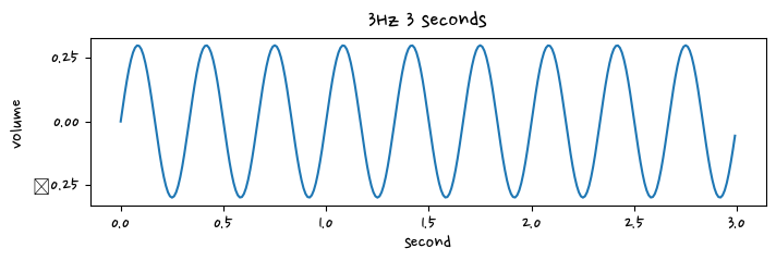
f =3
amp = 0.3
signal_2 = amp * np.sin(2*np.pi * f* t)plt.figure(figsize=(8,2))
plt.plot(t, signal_2)
plt.title("30% volume 3Hz 3 seconds")
plt.xlabel("second")
plt.ylabel("volume")
plt.show()
f =3
amp = 0.3
signal_3 = amp * np.sin(2*np.pi * f* t)
plt.figure(figsize=(8,2))
plt.plot(t, signal_3)
plt.title("20% volume 5Hz 3 seconds")
plt.xlabel("second")
plt.ylabel("volume")
plt.show()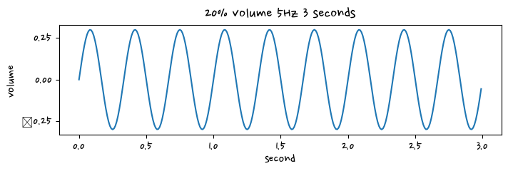
signal_1 = 1.0 * np.sin(2*np.pi * t)
plt.figure(figsize=(8,2))
plt.plot(t, signal_1)
plt.title("1Hz 3 seconds")
plt.xlabel("second")
plt.ylabel("volume")
plt.ylim(-1.2, 1.2)
plt.show()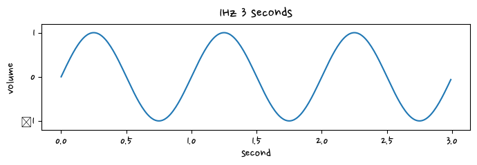
f = 5
amp = 0.2
signal_3 = amp * np.sin(2*np.pi * f* t)
plt.figure(figsize=(8,2))
plt.plot(t, signal_3)
plt.title("20% volume 5Hz 3 seconds")
plt.ylim([-1.2, 1.2])
plt.xlabel("second")
plt.ylabel("volume")
plt.show()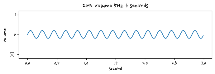
plt.figure(figsize=(8,2))
plt.plot(t, signal_1)
plt.plot(t, signal_2)
plt.plot(t, signal_3)
plt.title(["100% vol 1Hz 3sec ", "30% vol 3Hz 3 sec","20% volume 5Hz 3 seconds"])
plt.ylim([-1.2, 1.2])
plt.xlabel("second")
plt.ylabel("volume")
plt.show()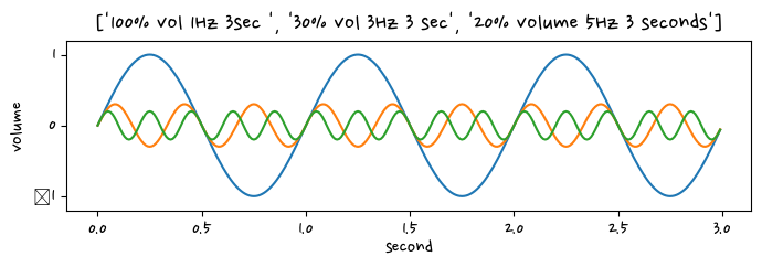
plt.figure(figsize=(8,4))
plt.plot(t, signal_1+signal_2+signal_3)
plt.title(["100% vol 1Hz 3sec ", "30% vol 3Hz 3 sec","20% volume 5Hz 3 seconds"])
plt.ylim([-1.2, 1.2])
plt.xlabel("second")
plt.ylabel("volume")
plt.show()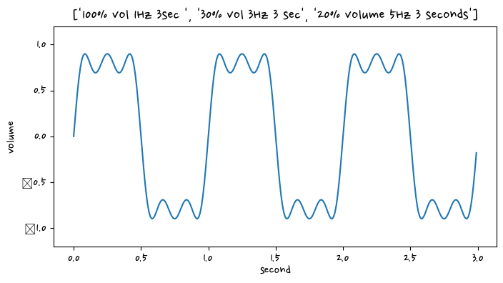
df = fs / N #주파수 간격
f = np.arange(0, N)
signals = signal_1+signal_2+signal_3
Xf = np.fft.fft(signals)
plt.subplot(121)
plt.plot(f, np.abs(Xf), "o")

plt.subplot(122)
plt.plot(f[:int(N/2)], np.abs(Xf[:int(N/2)]), "o")
plt.show()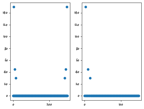Xf[:5] #-9.49612074e-16+0.00000000e+00j = 복소수array([-9.49612074e-16+0.00000000e+00j, -6.49443331e-15-2.33146835e-15j,
2.45253753e-14+1.11465716e-15j, -2.30463730e-14-1.50000000e+02j,
2.72803434e-14-1.96798384e-15j])Nyquist sampling theory
f = 20 # hz
t = np.linspace(0, 0.5, 200)
x1 = np.sin(2.0*np.pi*f*t)
fs = 35 #hz
T = 1/fs
n = np.arange(0, 0.5/T)
nT = n * T
x2 = np.sin(2.0*np.pi*f*nT) plt.subplot(221)
plt.plot(t, x1)
plt.subplot(222)
plt.plot(t, x1)
plt.plot(nT, x2, "o")
plt.subplot(223)
plt.plot(t, x1)
plt.plot(nT, x2, "-o")
plt.show()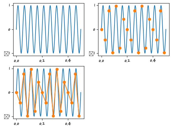
f = 20 # hz
t = np.linspace(0, 0.5, 200)
x1 = np.sin(2.0*np.pi*f*t)
fs = 60 #hz
T = 1/fs
n = np.arange(0, 0.5/T)
nT = n * T
x2 = np.sin(2.0*np.pi*f*nT) plt.subplot(221)
plt.plot(t, x1)
plt.subplot(222)
plt.plot(t, x1)
plt.plot(nT, x2, "o")
plt.subplot(223)
plt.plot(t, x1)
plt.plot(nT, x2, "-o")
plt.show()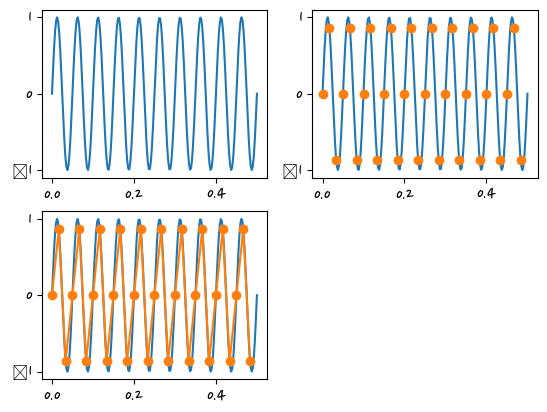
fs = 100 #샘플링 주파수
dt = 1/fs #샘플 간 시간
N = 300 # 샘플 개수(3초)
t = np.arange(0,N) * dt
signals=0
amp=1
for f in range(1, 60+1):
    signals += amp[i] * np.sin(2*np.pi * f *t)
plt.figure(figsize=(8,2))
plt.plot(t, signals)
plt.xlabel("second")
plt.ylabel("volume")
plt.show()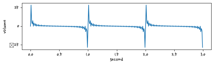
fs = 100 #샘플링 주파수
dt = 1/fs #샘플 간 시간
N = 300 # 샘플 개수(3초)
t = np.arange(0,N) * dt
signals=0
amp=1
for f in range(1, 60+1):
    signals += amp * np.sin(2*np.pi * f *t)
plt.figure(figsize=(8,2))
plt.plot(t, signals)
plt.xlabel("second")
plt.ylabel("volume")
plt.show() 
fs = 100 #샘플링 주파수
dt = 1/fs #샘플 간 시간
N = 300 # 샘플 개수(3초)
t = np.arange(0,N) * dt
signals=0
amp=[1, 0, 0.3, 0., 0.3, 0,0,0,0,0]
for f, amp_val in enumerate(amp):
    f = f+1
    signals += amp_val * np.sin(2*np.pi * f *t)
plt.figure(figsize=(8,2))
plt.plot(t, signals)
plt.xlabel("second")
plt.ylabel("volume")
plt.show()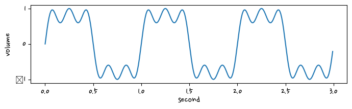

DL 공부중
🐱