Ch5. 구매 요인 분석 (Decision Tree)
- Gini Index
- Decision Tree 설명
- Decision Tree VS Logistic Regression
- DT:
- Non Parametric
- Feature Power X
- Categorical Value O
- LR:
- Parametric
- Feature Power O
- Categorical Value X
- DT:
Ch6. 프로모션 효율 예측 (Random Forest)
- Class Imbalance Problem
- Confusion Matrix
- Sklearn Classfication Report
- Overfitting
- Bagging
- Random Sampling (sampling with replacement)
- Tree Voting System
- Random Forest
- Independent variable Sampling
- Better result than Baggin method
- suppress super variable
- Check Feature Importance
Ch7. 고객 분류 (KMeans)
- Machine Learning
- Supervised Learning
- Classification, Regression
- Unsupervised Learning
- Clustering, Dimensionality Reduction
- Reinforcement Learning
- Supervised Learning
- [KMeans] How to select number of clusters?
- inertia ⇒ 그룹에 포함된 데이터들이 퍼져있는 정도
- 각 클러스터의 중심인 centroid와 각 데이터들 사이의 거리를 나타냄
- Inertia가 낮을수록 좋은 그룹
- Plot Elbow Method
- 그래프가 Smooth한 경우 ⇒ 애매함 (Silhouette Score 활용)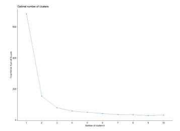
- Silhouette Score
- 개체가 다른 클러스터(seperation)에 비해 자신의 클러스터(cohesion)와 얼마나 유사한 측정
- 군집의 수가 많다고 Score가 높아지지 않음
- [-1, 1]
- 값이 높으면 객체가 자체 클러스터와 잘 일치하고 인접 클러스터와 잘 일치하지 않음
- inertia ⇒ 그룹에 포함된 데이터들이 퍼져있는 정도
- PCA
- Dimensionality reduction method
Ch8. 쇼핑몰 매출 예측 (Time Series)
-
Preprocessing: Python datetime library, pandas date api
-
Linear Regression
-
Pandas print option
import pandas as pd pd.set_option('display.float_format', lambda x: '%.0f' % x) -
Unix time stamp
-
Time Series data preprocessing
- Group montly, daily
- pd.resample
- M: group by month end (ex. 2022-05-31)
- MS: group by month start (ex. 2022-05-01)
-
pystan, fbprophet, plotly
-
fbprophet
-
condition
- 1년 이상의 데이터 (최소 1달)
- Seasonality
- event/holiday 지정 할 수 있음
- historical trend change 명확할 수록 성능이 좋음
-
column rename
- date column name : ds
- time value: yfrom fbprohet import Prophet model = Prophet() model.fit(df) future = model.make_future_dataframe(periods=12, freq='MS') # 1년치 데이터 pred = model.predict(future) model.plot(pred) plt.show()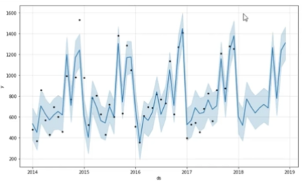
-
result
- ds
- yhat: predict result
- yhat_lower
- yhat_upper
-
model.plot_components(pred); plt.show()
- trend
- seasonality
-
-
-
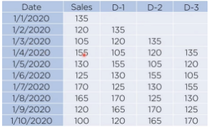
AR model
from statsmodels.tsa.ar_model import AutoReg model = AutoReg(data, lags=12) model_fit = model.fit() pred = model_fit.predict(start=start_date_index, end=end_date_index)- Data가 단순한 경우 사용 가능
- Prophet보다는 예측 성능이 떨어짐
- 원리
-
feature를 lag로 활용함
-
-
Time series 구성요소
- Trend: 추세 (증가, 감소 등..)
- Seasonality: 계절성 (특정 주기 패턴)
- Cyclic: 장기적인 변화
- Irregularity: 잔차(오류)
- 많은 비중을 차지할 경우 ⇒ 예측이 매우 어려움
Ch9. 상품 리뷰 분석 (NLP)
- nltk library
- stopwords
- wordclound
-
단어의 빈도수에 따라, 더 자주 등장하는 단어를 더 크고 굵게 보여주는 visualization 기법
-
활용 사례
- Finding Pain Points
- SEO
- 관련 주요 키워드를 확인하여, 사이트를 검색 결과에 더욱 잘 노출시키도록 개선from wordcloud import WordCloud wc = WordCloud().generate(str(data['text'])) plt.figure(figsize=(10,5)) plt.imhow(wc) plt.axis('off')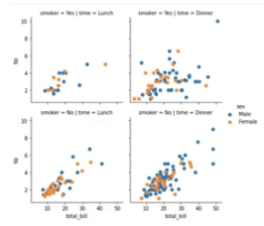
-
- sklearn CountVectorizer
- 단어별 빈도를 계산하여 데이터 프레임으로 정리
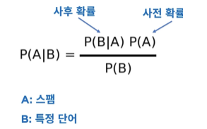
- Naive Bayes
-
각 변수가 독립적이라는 가정
-
n < p 일 때, 유용하게 쓰임
-
딥러닝을 제외하면, 텍스트 데이터에 가장 적합 (스팸 메일 필터링, 감정 분석)
-
Ch10. GA 데이터 적용 시나리오
- BigQuery
# conda install pandas-gbq -c conda-forge from pandas.io import gbq - Json format Data
# json 포맷으로 바로 변경 (device 칼럼에 json 형식으로 데이터가 저장됨) pd.read_csv('ga.csv', converters= {column: json.loads for column in json_columns}) # json normalize -> json 포맷이 pandas Dataframe으로 변환됨 json_normalize(data['device']) - logarization
Ch11. 데이터 시각화 (Visualization)
-
matplotlib
fig = plt.figure() axes1 = fig.add_axes([0.1, 0.1, 0.9, 0.9]) axes2 = fig.add_axes([0.2, 0.6, 0.3, 0.3]) axes1.plot(x, y, 'r') axes1.plot(y, x, 'b') fig, axes = plt.subplots(nrow=2, ncol=3) -
seaborn
- distribution plot
- displot
- jointplot
- pairplot
- rugplot
- categorical plot
- countplot
- boxplot
- violinplot
- matrix plot
- heatmap
- clustermap: 특성이 비슷한 것끼리 재배열
- grid plot
-
FacetGrid
g = sns.FacetGrid(data, col='time', row='smoker')
g = g.map(plt.scatter, 'total_bill').add_legend()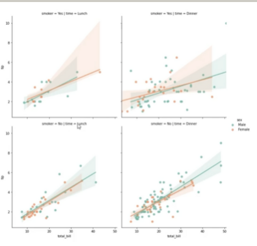
-
- regression plot
-
lmplot
sns.lmplot(x='total_bill', y='tip', data=data, hue='sex', col='time', row='smoker', palette='Set2')
-
- distribution plot

Data Scientist, Data Analyst