지금까지 읽었던 real time system 관련 논문 중에서는 읽는 데 가장 오래 걸렸던 것 같다. scheduling model의 periodic capacity bound를 구하고 이를 기반으로 single periodic workload로 추상화하는 개념이 신기했다. 역시 똑똑한 사람은 정말 많다..
Introduction
scheduling model은 보통 3가지의 요소로 이루어져있음
a resource model
a scheduling algorithm
a workload model
hierarchical scheduling interface model I(GS,GD)
GS : real-time guarantee that parent node supplies to the child node
GD : real-time guarantee that child node demands to the parent node
W → workload model - L&L tasks (period, execution time)
R → resource model - partitioned resource model
A → scheduling algorithm - RM / EDF
scheduling algorithm M is said to be scheduable if W is schedulable under A with R
Periodic Resource Model Γ(Π,Θ) → Π time unit마다 Θ time unit만큼 리소스 쓸 수 있다고 개런티
Exact schedulability : necessary and sufficient 하게 schedulable하지 않은지 확인 가능해야함
Periodic capacity bound : scheduling algorithm M에서 schedulable smallest possible periodic capacity bound를 (Θ∗/Π) 라고 했을 때 Θ≥Θ∗ 여야함
Utilization bound : the largest possible utilization bound UB(≥∑Ti∈Wpiei)를 찾아야 함
Algorithm set : a set of algorithms A( has schedulable algorithm A) 찾기
Compositional guarantee : parant scheduling이 schedulable하다면, iff 그를 구성하는 n개의 child model도 schedulable하다.
Periodic Resource Model
periodic resource model Γ(Π,Θ) → 매 Π 시간마다 Θ 시간 만큼의 resource allocation 보장
Γ(k,k)는 항상 이용가능한 dedicated resource라는 의미 (k 시간마다 k시간 만큼 가능하다는거니까)
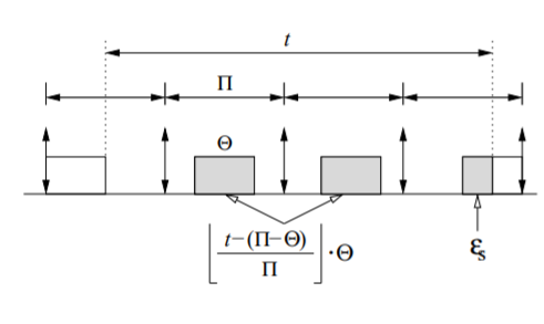
✔ Resource supply
→ the amount of resource allocations that the resource provides
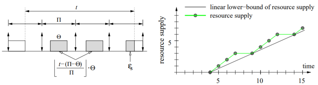
minimum resource supply bound function sbfΓ(t)=⌊Πt−(Π−Θ)⌋⋅Θ+ϵs
where ϵs=max(t−(Π−Θ)−⌊Πt−(Π−Θ)⌋−(Π−Θ),0)
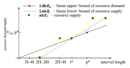
linear supply bound function (lower bound of sbfΓ(t)) lsbfΓ(t)=ΠΘ(t−2⋅(Π−Θ))≤sbfΓ(t)
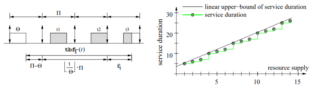
✔ Service time
→ the duration that it takes for the resource to provide a resource supply
maximum service time bound function (for t time unit supply) tbfΓ(t)=(Π−Θ)+Π⋅⌊Θt⌋+ϵt
where ϵs={Π−Θ+t−Π⌊Θt⌋0if (t−Θ⌊Θt⌋>0)otherwise
linear service time bound function (upper bound of tbfΓ(t)) ltbfΓ(t)=ΘΠ⋅t+2(Π−Θ)≥tbfΓ(t)
Schedulability Analysis
이 장에서는 scheduling model M(W,Γ,A)이 주어졌을 때 이 scheduling model이 schedulable한지 확인한다.
Schedulability Analysis under EDF Scheduling
✔ Resource demand
→ the amount of resource allocation that the workload set requests
maximum resource demand bound function (of time interval length t under EDF) dbfW(t)=Ti∈W∑⌊pit⌋⋅ei
linear demand bound function (upper bound of dbfW(t)) ldbfW(t)=UW⋅t≥dbfW(t) where UW is utilization of the workload set W
dedicated resource라고 할 때, hyperperiod에서의 resource demand ≤ the length of the time interval이면 schedulable 하다.
여기에서 t time에 대한 resource demand는 변하지 않지만 partitioned resource를 표현하기 위해서 우변이 바뀔 필요가 있음
아까 구해뒀던 sbfΓ(t) -minimum resource supply bound function-로 우변을 바꿀 수 있음
Theorem 1. For a given scheduling model M(W,Γ,EDF), M is schedulable iff the resource demand of W during a time interval is no greater than the resource supply of Γ during the same time interval for all time interval during a hyperperiod, i.e., ∀0<t≤2⋅LCMW:dbfW(t)≤sbfΓ(t).
Schedulability Analysis under Fixed-Priority Scheduling
scheduling model M′(W,Γ(1,1),FP) -dedicated resource- 에 대해서 M′은 iff WCRT(Worst-Case Response Time) ≤ its relative deadline 일 때 schedulable하다.
ri의 WCRT는 나보다 더 높은 priority들이 전부 동시에 들어오는 critical instant에 발생한다. ri를 구하는 iterative algorithm ↓
ri(k)=ei+Tk∈HP(W,T)∑⌊pkrik−1⌋⋅ek where Tk=(pk,ek)
(dedicated resource 상황-t time의 resource supply를 얻기위한 service duration이 t time-에서) 나보다 높은 priority(HP)에 의해 preemption되는 시간을 반복적으로 구하는 알고리즘이다.
periodic partitioned resource Γ(Π,Θ)을 고려한 WCRT를 구하는 식을 구하면
ri(k)(Γ)=tbfΓ(Ii(k)) where Ii(k)=ei+Tk∈HP(W,T)∑⌈pkri(k−1)(Γ)⌉⋅ek
Theorem 2. For a given scheduling model M(W,Γ,FP), where FP is a fixed-priority algorithm, M is schedulable iff ∀Ti∈W:ri(Γ)≤pi,whereTi=(pi,ei).
Schedulability Bounds
Periodic Capacity Bounds
periodic resource Γ(Π,Θ)의 periodic capacity CΓ를 Θ/Π 로 정의할 수 있음
그러면 periodic capacity bound PCBW(Π,A)≤ΠΘ 을 만족할 때 schedulable한 PCBW를 정의할 수 있다.
single periodic workload T(p,e)를 p=Π, e=Π⋅PCBW(Π,A)로 추상화할 수 있다..
✔ Periodic Capacity Bound for EDF scheduling
Theorem 3. For a given periodic workload set W under EDF scheduling algorithm, the optimal(minimum) periodic capacity bound PCBW∗(Π,EDF) of a period is PCBW∗(Π,EDF)=ΠΘ∗ where Θ∗ is smallest possible Θ satisfying ∀0<t≤2⋅LCMW:dbfW(t)≤sbfΓ(t)
A scheduling model M(W,Γ(Π,Θ),EDF) is schedulable iff PCBW∗(Π,EDF)≤CΓ.
Theorem 4. For a given periodic workload set W under EDF scheduling algorithm, a periodic capacity bound PCBW(Π,EDF) of a resource period Π is PCBW(Π,EDF)=ΠΘ+ where Θ+=0<t≤2LCMwmax(4(t−2Π)2+8ΠdbfW(t)−(t−2Π))
dbfW(t)≤lsbfΓ(t)=ΠΘ(t−2Π+2Θ)≤sbfΓ(t) 이므로 근의 공식을 이용해 최소 Θ의 값을 찾을 수 있다.
✔ Periodic Capacity Bound for RM scheduling
Theorem 5. For a given periodic workload set W under RM scheduling algorithm, the optimal(minimum) periodic capacity bound PCBW∗(Π,EDF) of a resource period Π for a periodic partition resource Γ isPCBW∗(Π,RM)=ΠΘ∗ where Θ∗ is smallest possible Θ satisfying ∀Ti∈W:ri(Γ)≤pi,whereTi=(pi,ei).
A scheduling model M(W,Γ(Π,Θ),RM) is schedulable iff PCBW∗(Π,RM)≤CΓ.
Theorem 6. For a given periodic workload set W under RM scheduling algorithm, a periodic capacity bound PCBW(Π,RM) of a resource period Π for a periodic partition resource Γ is PCBW(Π,RM)=ΠΘ+ where Θ+=∀Ti∈Wmax(4−(pi−2Π)+(pi−2Π)2+8ΠIi), where Ii=ei+Tk∈HP(W,T)∑⌊pkpi⌋⋅ek
∀Ti∈W:ltbfΓ(Ii)=ΘΠ⋅Ii+2(Π−Θ)≤pi 이므로 마찬가지로 근의 공식을 이용해 최소 Θ의 값을 찾을 수 있다.
Utilization Bounds
위에서 구했던 periodic capacity처럼, periodic resource Γ에 대해 아래의 조건을 만족해야 schedulable한 utilization bound UBΓ(A)를 정의할 수 있다.
interval length가 일정 값 이상으로 커지면, 그 값 이상에 대해서는 위의 대소관계가 항상 성립함을 알 수 있다.
Theorem 7. Given a periodic resource Γ(Π,Θ), a utilization bound UBΓ(EDF) of the EDF algorithm for a periodic workload set W is UBΓ(EDF)=ΠΘ(1−p∗2(Π−Θ)) where p∗ is the smallest period in the workload set W.
✔ Utilization Bound for RM scheduling
Theorem 8. Given a periodic resource Γ(Π,Θ), a utilization bound UBΓ(RM) of the RM algorithm for a set of m periodic workload is UBΓ(RM)=ΠΘ(m(m2−1)−p∗m2(Π−Θ)) where p∗ is the smallest period in the workload set W.
Compositional Real-Time Guarantees & Conclusions
Definition. Given multiple scheduling models M1,…,Mn, we derive a scheduling model MP(WP,ΓP,AP) from M1,…,Mn as follows.
1. we assume that AP and ΠP are given
2. we derive WP by simply mapping the resource model of a child scheduling model Γi(Πi,Θi) to its periodic task Ti(pi,ei) such that WP={T1(Π1,Θ1),…,Tn(Πn,Θn)}.
3. we first derive PCBWP∗(ΠP,AP) according to Theorem 3 or Theorem 5 depending on AP. If PCBWP∗(ΠP,AP) is derived, we then compute ΘP such that ΘP=ΠP⋅PCBWP∗(ΠP,AP).
Theorem 9. Given multiple scheduling models M1,…,Mn that are individually schedulable, we derive a scheduling model MP(WP,ΓP,AP) from M1,…,Mn according to the composition method in above Definition. Then, we construct a hierarchical schduling framework H such that MP is a parent scheduling model of M1,…,Mn. H supports the compositional real-time guarantees such that MP is schedulable, iff M1,…,Mn are schedulable in the framework.
Π time마다 최소 Θ time만큼 사용할 수 있는 partitioned resource를 가진 scheduling model을 주기 Π마다 execution time이 Θ인 하나의 task로 추상화

잘 보고 갑니다 ㅎㅎ 흥미로운 내용이네요 앞으로도 많은 포스팅 부탁드려요