---

1. Introduction

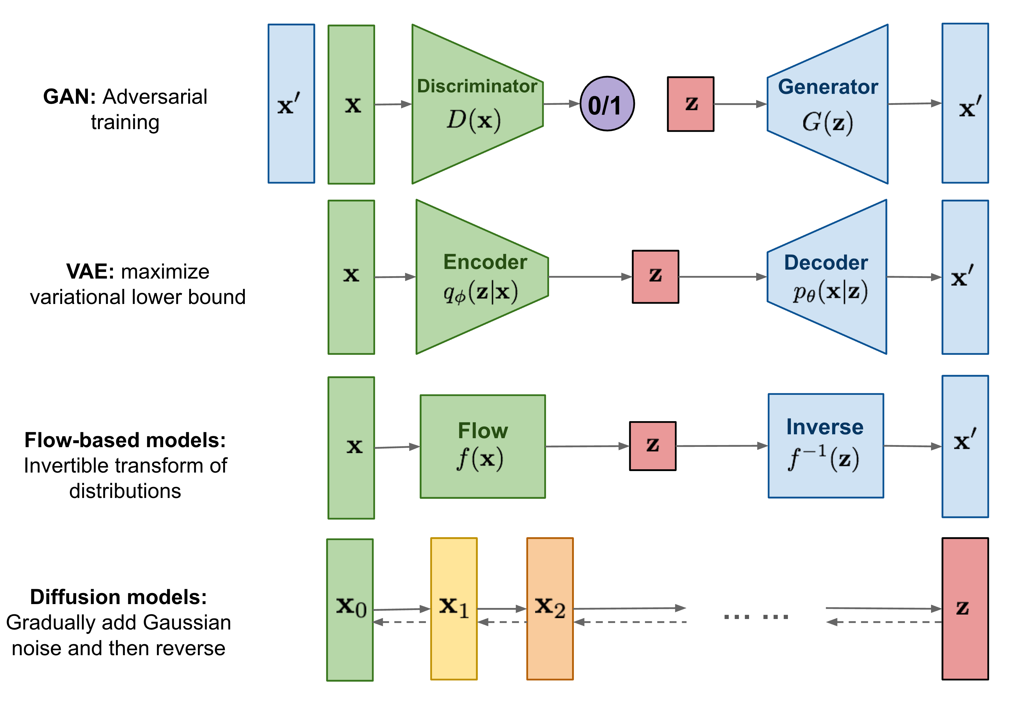
Diffusion model은 variational inference로 학습시켜 데이터를 생성하는 parameterized Markov chain. Diffusion model은 Markov가 데이터가 normal distribution의 형태를 할 때까지 noise를 더해가는 diffusion process와 이를 역으로 거치며 학습하는 reverse process로 구성됨.

Diffusion model은 정의하기 쉽고 학습시키는 것도 편리함. 또한 높은 품질의 sample(output)도 생성이 가능.

• Variational inference(변분추론): 사후확률(posterior) 분포 $p(z |x)$를 다루기 쉬운 확률분포 $q(z)$로 근사(approximation)하는 것
• Parameterize: 하나의 표현식에 대해 다른 parameter를 사용하여 다시 표현하는 과정. 이 과정에서 보통 parameter의 개수를 표현 식의 차수보다 적은 수로 선택(ex. 3차 표현식 --> 2개 parameter 사용)하므로, 낮은 차수로의 mapping 함수(ex. 3D --> 2D)가 생성
• Markov chain: 어떤 상태에서 다른 상태로 넘어갈 때, 바로 전 단계의 상태에만 영향을 받는 확률 과정

---

2. Background

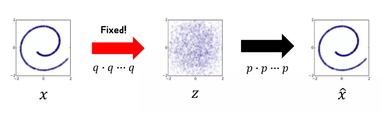
2-1. Forward(diffusion) process $q(\mathbf{x}_t|\mathbf{x}_{t-1})$

Markov chain으로 data에 noise를 추가하는 과정. Noise를 추가할 때 variance schedule $\beta_1,,,\beta_T$로 scaling을 한 후 더해준다.

• $\beta_t = 1$이면 mean인 $\sqrt{1-\beta_t}\mathbf{x}_{t-1} = 0$. 이전 정보를 갖지 못하고 노이즈가 증가함
• 단순히 noise만을 더해주는게 아니라 $\sqrt{1-\beta_t}$로 scaling하는 이유는 variance가 발산하는 것을 막기 위함
• $q(x_1|x_0)$: $x_0$에 noise를 추가해 $x_1$을 만드는 과정
• $x_T$는 완전 destroy된 noise 상태 ~ $N(x_T;0, I)$

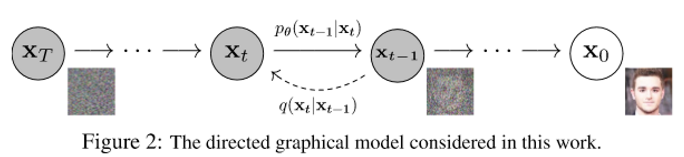
2-2. Reverse process $p(\mathbf{x}_{t-1}|\mathbf{x}_t)$

Reverse process로 가우시안 노이즈를 사용하는 이유는 1994년 논문에 forward process가 가우시안이면 reverse process도 가우시안으로 쓰면 된다라는 증명이 있다고 함.

여기서 우리가 해야 할 것은 $\mathbf{x}_t$를 보고 $\mathbf{x}_{t-1}$의 평균 $\mu_\theta$과 분산 $\Sigma_\theta$을 예측해내는 것.

• Hierarachical VAE에서의 decoding 과정과 비슷함
• $\mu_\theta$과 분산 $\Sigma_\theta$는 학습 가능한 parameter

2-3. Loss Function $L$

Diffusion model의 목적은 noise를 어떻게 제거할 것인가?이다. $x_t$가 들어왔을 때 $x_{t-1}$을 예측할 수 있다면 $x_0$ 또한 예측이 가능해짐.

본 논문에서는 negative log likelihood를 최소화하는 방향으로 진행. 위 수식을 ELBO(Evidence of Lower BOund)로 우항과 같이 정리하고 이를 풀어내면

ELBO의 역할은 우리가 관찰한 P(z|x)가 다루기 힘든 분포를 이루고 있을 때 이를 조금 더 다루기 쉬운 분포인 Q(x)로 대신 표현하려 하는 과정에서 두 분포 (P(z|x)와 Q(x))의 차이 (KL Divergence)를 최소화 하기 위해 사용된다.

와 같은 결과가 나온다.

• $L_T$: Regularization term으로 $\beta_t$를 학습시킴
• $L_{t-1}$: Reconstruction term으로 매 단계에서 noise를 지우는 지움
• $L_0$: Reconstruction term으로 최종 단계에서 image를 생성

---

3. Diffusion models and denoising encoders

DDPM에서는 inductive bias를 늘려 모델을 더 stable하고 성능도 개선할 수 있었음.

Inductive bias: 학습 모델이 지금까지 만나보지 못했던 상황에서 정확한 예측을 하기 위해 사용하는 추가적인 가정, 즉 우리가 풀려는 문제에 대한 정보를 모델에 적용하는 것

3-1. Forward process and $L_T$

$\beta_t$를 고정했더니 학습이 잘됨. 10^-4 ~ 0.02로 linear하게 image에 가까울수록 noise를 적게 주는 방식으로 설정.

따라서 $q$에는 학습 가능한 parameter가 없어 $L_T$는 0이 되기 때문에 삭제할 수 있었음.

3-2. Reverse process and $L_{1:T-1}$

• $q\left(x_{t-1} \mid x_t, x_0\right)=N\left(x_{t-1} ; \tilde{\mu}\left(x_t, x_0\right), \tilde{\beta}_t \mathrm{I}\right)$
• $p_\theta\left(x_{t-1} \mid x_t\right)=\mathcal{N}\left(x_{t-1} ; \mu_\theta\left(x_t, t\right), \sum_\theta\left(x_t, t\right)\right)$

$L_{1:T-1}$는 forward progress posterior를 예측하는 loss. $\mathbf{x}_{t-1}$에서 noise를 더해 $\mathbf{x}_{t}$를 만들었을때, 그 과정을 복원 $p(\mathbf{x}_{t-1}|\mathbf{x}_t)$ 하는 과정을 학습.

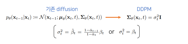
• $\Sigma_\theta$: $\beta$를 상수로 가정했고 $p(\mathbf{x}_{t-1}|\mathbf{x}_t)$의 variance가 $\beta$에 영향을 받기 때문에 학습시키지 않아도 된다고 생각해 variance term을 제거함.

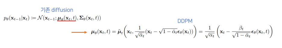
• $\mu_\theta$: DDPM에서는 $\mu_\theta$를 바로 구하지 않고 residual $\epsilon_\theta$만 구해 정확도를 높임.

3-3. Data scaling, reverse process decoder and $L_0$

[0, 255]의 image를 [-1,1] 사이로 linearly mapping. Sampling 마지막 단계에는 noise를 추가하지 않음.

$L_0$은 두 normal distribution 사이의 KL divergence를 나타냄.

• $D$: Data dimensionality
• $i$: 좌표

3-4. Simplified training objective

최종 loss는 위와 같이 나타난다. Ground truth - estimated output간 MSE loss를 줄이는 과정이 denoising과 비슷해 DDPM이라는 이름이 붙음.

Simplified objective을 통해 diffusion process를 학습하면 매우 작은 t 에서뿐만 아니라 큰 t에 대해서도 network 학습이 가능하기 때문에 매우 효과적.

• Algorithm 1: Training
  • Noise를 더해나가는 과정, network($\epsilon_\theta$, $p_\theta$)가 t step에서 noise($\epsilon$)가 얼마만큼 더해졌는지를 학습한다.
  • 학습 시에는 특정 step의 이미지가 얼마나 gaussian noise가 추가되었는지를 예측하도록 학습된다.
  • 코드에서는 랜덤 노이즈와 시간 단계 t로 노이즈가 추가된 이미지를 얻고 해당 이미지를 보고 모델이 노이즈를 예측

def p_losses(self, x_start, t, noise = None):
        b, c, h, w = x_start.shape
        noise = default(noise, lambda: torch.randn_like(x_start))

        # noise sample

        x = self.q_sample(x_start = x_start, t = t, noise = noise)

        # if doing self-conditioning, 50% of the time, predict x_start from current set of times
        # and condition with unet with that
        # this technique will slow down training by 25%, but seems to lower FID significantly

        x_self_cond = None
        if self.self_condition and random() < 0.5:
            with torch.no_grad():
                x_self_cond = self.model_predictions(x, t).pred_x_start
                x_self_cond.detach_()

        # predict and take gradient step

        model_out = self.model(x, t, x_self_cond)

        if self.objective == 'pred_noise':
            target = noise
        elif self.objective == 'pred_x0':
            target = x_start
        elif self.objective == 'pred_v':
            v = self.predict_v(x_start, t, noise)
            target = v
        else:
            raise ValueError(f'unknown objective {self.objective}')

        loss = self.loss_fn(model_out, target, reduction = 'none')
        loss = reduce(loss, 'b ... -> b (...)', 'mean')

        loss = loss * extract(self.loss_weight, t, loss.shape)
        return loss.mean()

• Algorithm 2: Sampling
  • Network를 학습하고 나면, gaussian noise에서 시작해서 순차적으로 denoising 하는 것이 가능하다. (by parameterized markovian chain)
  • 코드에서는 noise 제거 후 소량의 noise를 다시 추가하고 있음

@torch.no_grad()
def p_sample(self, x, t: int, x_self_cond = None):
    b, *_, device = *x.shape, x.device
    batched_times = torch.full((b,), t, device = x.device, dtype = torch.long)
    model_mean, _, model_log_variance, x_start = self.p_mean_variance(x = x, t = batched_times, x_self_cond = x_self_cond, clip_denoised = True)
    noise = torch.randn_like(x) if t > 0 else 0. # no noise if t == 0
    pred_img = model_mean + (0.5 * model_log_variance).exp() * noise
    return pred_img, x_start

4. Experiments

• T: 1000
• backbone: U-Net
  각 down/upsampling 단계는 ResNet/ConvNext 블록 2개 + (groupnorm + attention + residual) + down/upsampling으로 구성됨

block_klass = partial(ResnetBlock, groups = resnet_block_groups)

self.downs.append(nn.ModuleList([
                block_klass(dim_in, dim_in, time_emb_dim = time_dim),
                block_klass(dim_in, dim_in, time_emb_dim = time_dim),
                Residual(PreNorm(dim_in, LinearAttention(dim_in))),
                Downsample(dim_in, dim_out) if not is_last else nn.Conv2d(dim_in, dim_out, 3, padding = 1)
            ]))
            
 self.ups.append(nn.ModuleList([
                block_klass(dim_out + dim_in, dim_out, time_emb_dim = time_dim),
                block_klass(dim_out + dim_in, dim_out, time_emb_dim = time_dim),
                Residual(PreNorm(dim_out, LinearAttention(dim_out))),
                Upsample(dim_out, dim_in) if not is_last else  nn.Conv2d(dim_out, dim_in, 3, padding = 1)
            ]))

class Unet(nn.Module):
    def __init__(
        self,
        dim,
        init_dim = None,
        out_dim = None,
        dim_mults=(1, 2, 4, 8),
        channels = 3,
        self_condition = False,
        resnet_block_groups = 8,
        learned_variance = False,
        learned_sinusoidal_cond = False,
        random_fourier_features = False,
        learned_sinusoidal_dim = 16
    ):
        super().__init__()

        # determine dimensions

        self.channels = channels
        self.self_condition = self_condition
        input_channels = channels * (2 if self_condition else 1)

        init_dim = default(init_dim, dim)
        self.init_conv = nn.Conv2d(input_channels, init_dim, 7, padding = 3)

        dims = [init_dim, *map(lambda m: dim * m, dim_mults)]
        in_out = list(zip(dims[:-1], dims[1:]))

        block_klass = partial(ResnetBlock, groups = resnet_block_groups)

        # time embeddings

        time_dim = dim * 4

        self.random_or_learned_sinusoidal_cond = learned_sinusoidal_cond or random_fourier_features

        if self.random_or_learned_sinusoidal_cond:
            sinu_pos_emb = RandomOrLearnedSinusoidalPosEmb(learned_sinusoidal_dim, random_fourier_features)
            fourier_dim = learned_sinusoidal_dim + 1
        else:
            sinu_pos_emb = SinusoidalPosEmb(dim)
            fourier_dim = dim

        self.time_mlp = nn.Sequential(
            sinu_pos_emb,
            nn.Linear(fourier_dim, time_dim),
            nn.GELU(),
            nn.Linear(time_dim, time_dim)
        )

        # layers

        self.downs = nn.ModuleList([])
        self.ups = nn.ModuleList([])
        num_resolutions = len(in_out)

        for ind, (dim_in, dim_out) in enumerate(in_out):
            is_last = ind >= (num_resolutions - 1)

            self.downs.append(nn.ModuleList([
                block_klass(dim_in, dim_in, time_emb_dim = time_dim),
                block_klass(dim_in, dim_in, time_emb_dim = time_dim),
                Residual(PreNorm(dim_in, LinearAttention(dim_in))),
                Downsample(dim_in, dim_out) if not is_last else nn.Conv2d(dim_in, dim_out, 3, padding = 1)
            ]))

        mid_dim = dims[-1]
        self.mid_block1 = block_klass(mid_dim, mid_dim, time_emb_dim = time_dim)
        self.mid_attn = Residual(PreNorm(mid_dim, Attention(mid_dim)))
        self.mid_block2 = block_klass(mid_dim, mid_dim, time_emb_dim = time_dim)

        for ind, (dim_in, dim_out) in enumerate(reversed(in_out)):
            is_last = ind == (len(in_out) - 1)

            self.ups.append(nn.ModuleList([
                block_klass(dim_out + dim_in, dim_out, time_emb_dim = time_dim),
                block_klass(dim_out + dim_in, dim_out, time_emb_dim = time_dim),
                Residual(PreNorm(dim_out, LinearAttention(dim_out))),
                Upsample(dim_out, dim_in) if not is_last else  nn.Conv2d(dim_out, dim_in, 3, padding = 1)
            ]))

        default_out_dim = channels * (1 if not learned_variance else 2)
        self.out_dim = default(out_dim, default_out_dim)

        self.final_res_block = block_klass(dim * 2, dim, time_emb_dim = time_dim)
        self.final_conv = nn.Conv2d(dim, self.out_dim, 1)
        
  def forward(self, x, time, x_self_cond = None):
          if self.self_condition:
              x_self_cond = default(x_self_cond, lambda: torch.zeros_like(x))
              x = torch.cat((x_self_cond, x), dim = 1)

          x = self.init_conv(x)
          r = x.clone()

          t = self.time_mlp(time)

          h = []

          for block1, block2, attn, downsample in self.downs:
              x = block1(x, t)
              h.append(x)

              x = block2(x, t)
              x = attn(x)
              h.append(x)

              x = downsample(x)

          x = self.mid_block1(x, t)
          x = self.mid_attn(x)
          x = self.mid_block2(x, t)

          for block1, block2, attn, upsample in self.ups:
              x = torch.cat((x, h.pop()), dim = 1)
              x = block1(x, t)

              x = torch.cat((x, h.pop()), dim = 1)
              x = block2(x, t)
              x = attn(x)

              x = upsample(x)

          x = torch.cat((x, r), dim = 1)

          x = self.final_res_block(x, t)
          return self.final_conv(x)

• 16 x 16 feature map resolution에 self-attention. conv에서 차원을 3배로 늘리고 q,k,v로 분해.

class Attention(nn.Module):
    def __init__(self, dim, heads = 4, dim_head = 32):
        super().__init__()
        self.scale = dim_head ** -0.5
        self.heads = heads
        hidden_dim = dim_head * heads

        self.to_qkv = nn.Conv2d(dim, hidden_dim * 3, 1, bias = False)
        self.to_out = nn.Conv2d(hidden_dim, dim, 1)

    def forward(self, x):
        b, c, h, w = x.shape
        qkv = self.to_qkv(x).chunk(3, dim = 1)
        q, k, v = map(lambda t: rearrange(t, 'b (h c) x y -> b h c (x y)', h = self.heads), qkv)

        q = q * self.scale

        sim = einsum('b h d i, b h d j -> b h i j', q, k)
        attn = sim.softmax(dim = -1)
        out = einsum('b h i j, b h d j -> b h i d', attn, v)

        out = rearrange(out, 'b h (x y) d -> b (h d) x y', x = h, y = w)
        return self.to_out(out)

• Linear attention

class LinearAttention(nn.Module):
    def __init__(self, dim, heads = 4, dim_head = 32):
        super().__init__()
        self.scale = dim_head ** -0.5
        self.heads = heads
        hidden_dim = dim_head * heads
        self.to_qkv = nn.Conv2d(dim, hidden_dim * 3, 1, bias = False)

        self.to_out = nn.Sequential(
            nn.Conv2d(hidden_dim, dim, 1),
            LayerNorm(dim)
        )

    def forward(self, x):
        b, c, h, w = x.shape
        qkv = self.to_qkv(x).chunk(3, dim = 1)
        q, k, v = map(lambda t: rearrange(t, 'b (h c) x y -> b h c (x y)', h = self.heads), qkv)

        q = q.softmax(dim = -2)
        k = k.softmax(dim = -1)

        q = q * self.scale
        v = v / (h * w)

        context = torch.einsum('b h d n, b h e n -> b h d e', k, v)

        out = torch.einsum('b h d e, b h d n -> b h e n', context, q)
        out = rearrange(out, 'b h c (x y) -> b (h c) x y', h = self.heads, x = h, y = w)
        return self.to_out(out)

• Diffusion time $T$는 각 residual block에 transformer sinusoidal positional embedding이 추가돼서 구분됨

class SinusoidalPosEmb(nn.Module):
    def __init__(self, dim):
        super().__init__()
        self.dim = dim

    def forward(self, x):
        device = x.device
        half_dim = self.dim // 2
        emb = math.log(10000) / (half_dim - 1)
        emb = torch.exp(torch.arange(half_dim, device=device) * -emb)
        emb = x[:, None] * emb[None, :]
        emb = torch.cat((emb.sin(), emb.cos()), dim=-1)
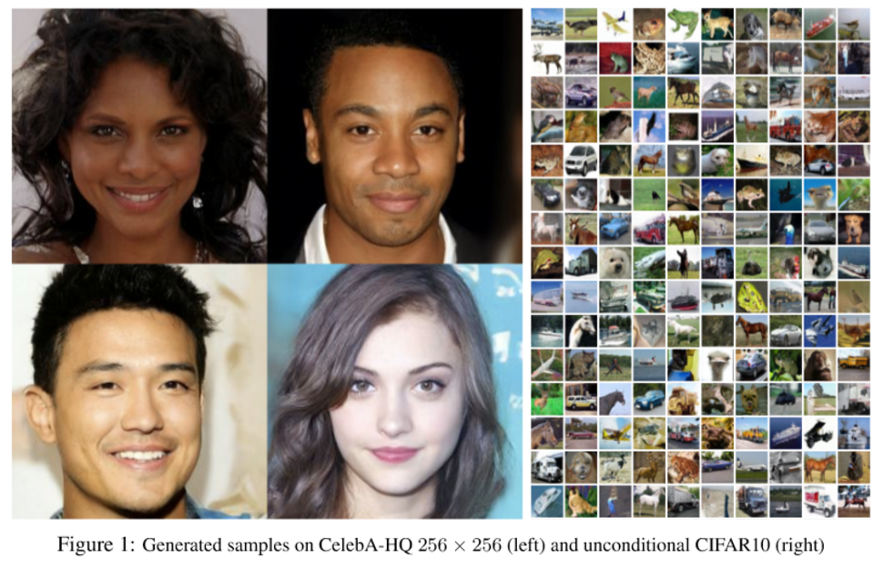
        return emb

4-1. Sample quality

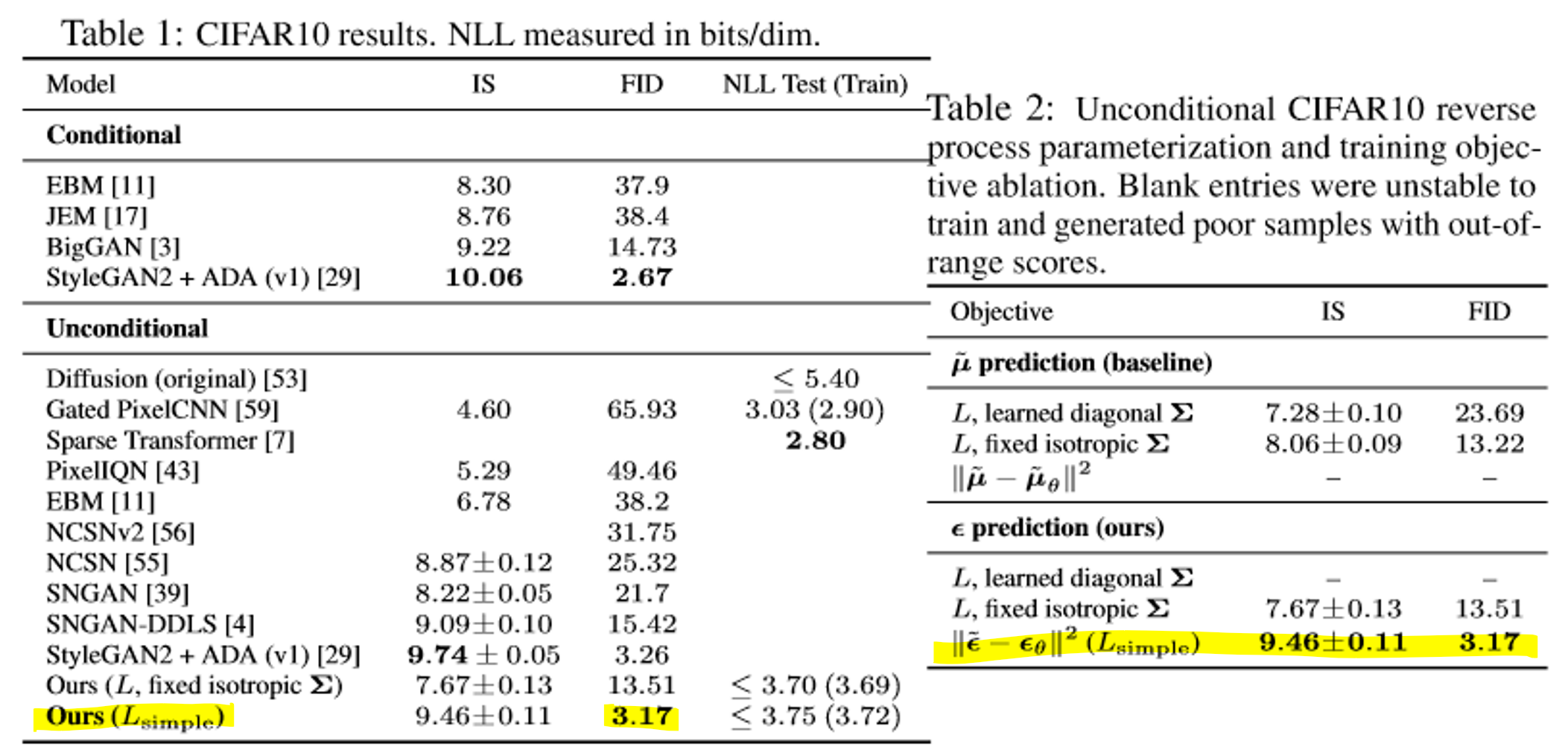
FID, IS로 metric 계산. Unconditional model인데도 conditional model보다 우월. Codelength에서 차이가 없기 때문에 overfitting의 가능성도 적음.

• FID score: Inception V3으로 이미지의 분포를 계산한 metric
• Unconditional model: 한번 dataset에 학습되면 추가적인 context 없이 image를 생성
• Conditional model: Class, label 등의 추가 정보를 받아 image를 생성

$\mu$보다 $\epsilon$을 계산하는 것이 성적이 좋고, fixed variance를 사용했을 때에도 성능이 감소하지 않음.

---

Questions

$N(x_T;0, I)$에서 I의 의미는?

• 단위행렬인것 같은데 왜 나오는지 모르겠음.

Noise를 만드는 과정이 fixed 돼있다면 그냥 매번 noise를 생성할 필요 없이 Gaussian dist.로 랜덤 생성하면 되는거 아닌가?

• Noise를 만드는 함수$q$의 분포에서 reverse process $p$를 유추하기 때문에 랜덤 생성하면 DDPM 자체가 성립하지 않을듯?

Markov chain의 n-1번째 상태는 n-2에 영향을 받았는데, n번째 상태는 n-2번째 상태와 독립적이라고 말할 수 있는가?

(Lossless) codelength는 무엇인가?

• Lossless codelength는 데이터의 엔트로피에 가까운 길이의 코드를 생성하는 데 사용되는 압축 알고리즘을 개발하는 것을 의미합니다. 이는 데이터의 분포에 대한 크로스 엔트로피를 최소화하여 생성 모델을 훈련시키고, 그 다음에 데이터의 엔트로피에 가까운 코드 길이를 갖는 코드를 구성하는 일반적인 방법입니다.

Reference

• 논문
  • Denoising Diffusion Probabilistic Models
• 코드
  • PyTorch implementation: denoising-diffusion-pytorch
  • 코드리뷰: Denoising Diffusion Pytorch
• 유투브
  • PR-409: Denoising Diffusion Probabilistic Models
• 논문 리뷰
  • [논문 리뷰] Denoising Diffusion Probabilistic Models
  • Score-Based / Diffusion Model[3] - DDPM
  • [논문리뷰] Denoising Diffusion Probabilistic Models (DDPM)
• 수식 증명
  • [논문공부] Denoising Diffusion Probabilistic Models (DDPM) 설명
  • [Paper Review] DDPM: Denoising Diffusion Probabilistic Models 논문 리뷰
  • [논문리뷰] DDPM: Denoising Diffusion Probabilistic Model
• etc.
  • ELBO (Evidence of Lower BOund)