1. 학습내용
- Numpy
- Pandas
2. 상세내용
# Numpy
## Numpy의 소개

NumPy(Numerical Python)는 파이썬에서 과학적 계산을 위한 핵심 라이브러리이다.
NumPy는 다차원 배열 객체와 배열과 함께 작동하는 도구들을 제공한다.
하지만 NumPy 자체로는 고수준의 데이터 분석 기능을 제공하지 않기 때문에 NumPy 배열과 배열 기반 컴퓨팅의 이해를 통해
pandas와 같은 도구를 좀 더 효율적으로 사용하는 것이 필요하다.
### ndarray 생성
array 함수를 사용하여 배열 생성하기import numpy as np# ndarray를 생성
arr = np.array([1,2,3,4])# print(arr) #[1 2 3 4]# type(arr) #numpy.ndarray
np.zeros((3,3))				array([	[0., 0., 0.],
       								[0., 0., 0.],
       								[0., 0., 0.] ])
# np.ones((3,3)) array([ [1., 1., 1.],
[1., 1., 1.],
[1., 1., 1.]])np.empty((4,4)) 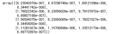
np.arange(10) #array([0, 1, 2, 3, 4, 5, 6, 7, 8, 9])
### ndarray 배열의 모양, 차수, 데이터 타입 확인하기

arr = np.array([[1,2,3],[4,5,6]])
arr.shape #(2, 3)arr.ndim #2arr.dtype #dtype('int32')arr_float = arr.astype(np.float64)print(arr_float) #[ [1. 2. 3.]
[4. 5. 6.]]
arr_float.dtype #dtype('float64')arr1 = np.array([[1,2],[3,4]])
arr2 = np.array([[5,6],[7,8]])
# arr3 = arr1 * arr2
# arr3 = np.add(arr1, arr2)
arr3 = np.multiply(arr1, arr2)
print(arr3) #[ [ 5 12]
[21 32] ]Numpy 배열의 연산은 연산자 (+,-,*,/)나 함수(add, subtract, multiply, divide)로 가능하다. ### ndarray 배열 슬라이싱 하기
ndarray 배열 슬라이싱 하기# 배열 슬라이싱
arr = np.array([[1,2,3],[4,5,6],[7,8,9]])
arr_1 = arr[:2, 1:3]
print(arr_1) #[ [2 3]
[5 6]]arr_1.shape #(2, 2)arr_int = np.arange(10)
# arr_int
print(arr_int[0:8:3]) #[0 3 6]print(arr[0,2]) #3arr = np.array([[1,2,3],[4,5,6]])idx = arr > 3
print(idx) #[[False False False]
[ True True True]]print(arr[idx]) #[4 5 6]import numpy as np##winequality-red.csv 파일 불러오기
redwine = np.loadtxt(fname = 'samples/winequality-red.csv', delimiter=';', skiprows = 1)redwine.shape #(1599, 12)print(redwine) 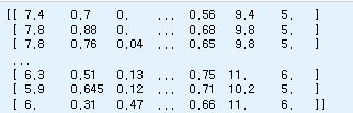
type(redwine) #numpy.ndarrayprint(redwine.sum()) #152084.78194print(redwine.mean()) #7.926036165311652print(redwine.mean(axis=0))
print(redwine[:,0].mean())               #8.31963727329581
#첫번째 축(0번 배열)에 대한것만 가져옴

# Pandas

## 자료구조 : Series와 Dataframe

Pandas에서 제공하는 데이터 자료구조는 Series와 Dataframe 두가지가 존재하는데 Series는 시계열과 유사한 데이터로서 index와 value가 존재하고 Dataframe은 딕셔너리데이터를 매트릭스 형태로 만들어 준 것 같은 frame을 가지고 있다. 이런 데이터 구조를 통해 시계열, 비시계열 데이터를 통합하여 다룰 수 있다.
## series

import pandas as pd
from pandas import Series, DataFrame

fruit = Series([2500,3800,1200,6000], index=['apple','banana','pear','cherry'])
fruit
print(fruit.values) #[2500 3800 1200 6000]print(fruit.index)
-> #Index(['apple', 'banana', 'pear', 'cherry'], dtype='object')fruitData = {'apple':2500, 'banana':3800, 'pear':1200, 'cherry':6000}
fruit = Series(fruitData)print(type(fruitData))
print(type(fruit))
fruit
fruit.name = 'fruitPrice'

fruit
fruit.index.name = 'fruitName'

fruit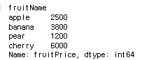
fruitData = {'fruitName':['apple','banana','pear','cherry'],
            'fruitPrice':[2500,3800,1200,6000],
            'num':[10,5,3,8]
            }

fruitName = DataFrame(fruitData)

fruitName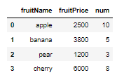
fruitFrame = DataFrame(fruitData, columns = ['fruitPrice','num','fruitName'])

fruitFrame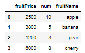
fruitFrame['fruitName']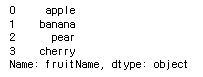
fruitFrame.fruitName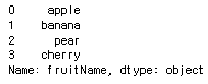
fruitFrame['Year'] = '2016'

fruitFrame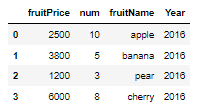
variable = Series([4,2,1], index=[0,2,3])
print(variable)
fruitFrame['stock'] = variable

fruitFrame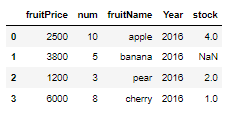
fruit = Series([2500,3800,1200,6000],index=['apple','banana','pear','cherry'])

fruit
new_fruit = fruit.drop('banana')
new_fruit
fruitData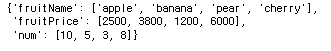
fruitName = fruitData['fruitName']
fruitName					#['apple', 'banana', 'pear', 'cherry']
fruitFrame = DataFrame(fruitData, index=fruitName, columns=['fruitPrice','num'])
fruitFrame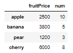
fruitFrame2 = fruitFrame.drop(['apple','cherry'])
fruitFrame2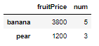
fruitFrame3 = fruitFrame.drop('num', axis=1)
fruitFrame3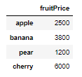
fruit
fruit['apple':'pear']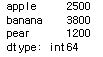
fruit[0:1]
fruitFrame['apple':'banana']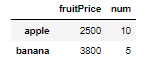
fruit1 = Series([5,9,10,3], index=['apple','banana','pear','cherry'])
fruit2 = Series([3,2,9,5,10], index=['apple','orange','banana','cherry', 'mango'])

fruit1 + fruit2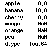
fruitData1 = {'Ohio' : [4,8,3,5],'Texas' : [0,1,2,3]}
fruitFrame1 = DataFrame(fruitData1,columns=['Ohio','Texas'],index = ['apple','banana','cherry','peer'])
fruitData2 = {'Ohio' : [3,0,2,1,7],'Colorado':[5,4,3,6,0]}
fruitFrame2 = DataFrame(fruitData2,columns =['Ohio','Colorado'],index = ['apple','orange','banana','cherry','mango'])
fruitFrame1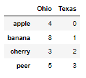
fruitFrame2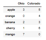
fruitFrame1 + fruitFrame2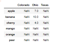
fruit
fruit.sort_values(ascending=False)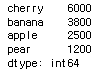
fruit.sort_index()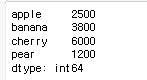
fruitFrame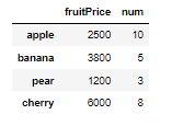
fruitFrame.sort_index()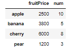
fruitFrame.sort_values(by=['fruitPrice','num'])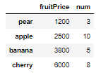
german = pd.read_csv('http://freakonometrics.free.fr/german_credit.csv')

german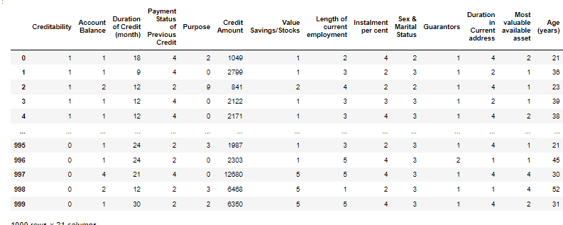
list(german.columns.values)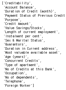
german_sample = german[['Creditability','Duration of Credit (month)','Purpose','Credit Amount']]german_sample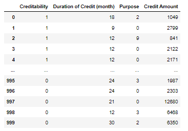
german_sample.min()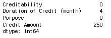
german_sample.max()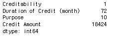
german_sample.mean()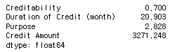
german_sample.describe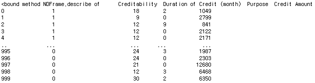
german_sample = german[['Duration of Credit (month)','Credit Amount','Age (years)']]german_sample.corr()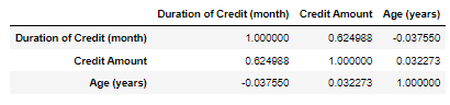
german_sample = german[['Credit Amount','Type of apartment']]

german_sample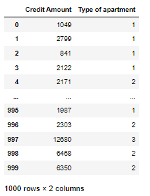
german_grouped = german_sample['Credit Amount'].groupby(
                 german_sample['Type of apartment']
)
german_grouped.mean()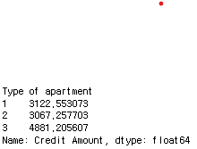
german_sample = german[['Credit Amount','Type of apartment','Purpose']]

german_grouped = german_sample['Credit Amount'].groupby(
     [german_sample['Purpose'],german_sample['Type of apartment']]
)
german_grouped

#<pandas.core.groupby.generic.SeriesGroupBy ~~
german_grouped.mean()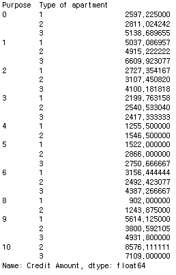
## Group간에 반복하기

한 개 그룹 반복
german=pd.read_csv("http://freakonometrics.free.fr/german_credit.csv")
german_sample=german[['Type of apartment','Sex & Marital Status','Credit Amount']]for type , group in german_sample.groupby('Type of apartment'):
print(type)
print(group.head(n=3))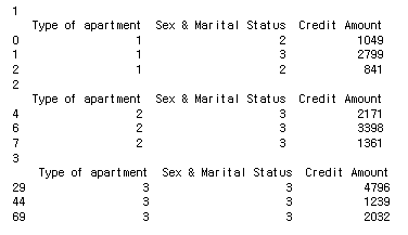
for (type,sex) , group in german_sample.groupby(['Type of apartment','Sex & Marital Status']):
    print((type,sex))
    print(group.head(n=3))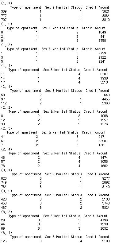
## 데이터 분석 예제 행성데이터

Seaborn 패키지에서 제공 받을 수 있는 행성 데이터 세트를 사용한다.
Seaborn 패키디는 천문학자가 다른 별 주변에서 발견한 행성에대 대한 정보를 제공하며 2014년까지 발견된 1000개 이상의 외계 행성에 대한 세부 정보를 담고 있다.
import seaborn as sns
planets = sns.load_dataset('planets')
planets.shape #(1035, 6)planets.head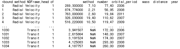
#dropna() 비여있는 값의 삭제
planets.dropna().describe()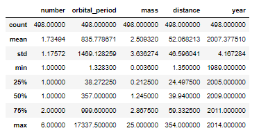
import pandas as pd

births = pd.read_csv('https://raw.githubusercontent.com/jakevdp/data-CDCbirths/master/births.csv')

births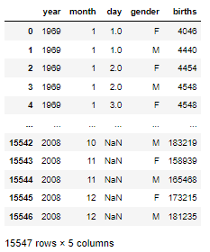
births.head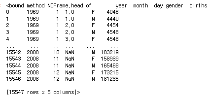
births['decade'] = (births['year']) // 10 * 10

births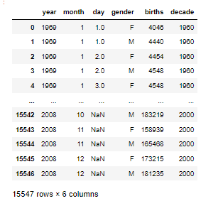
births.pivot_table('births', index='decade', columns='gender', aggfunc='sum')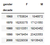
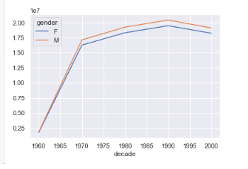
%matplotlib inline

import matplotlib.pyplot as plt

sns.set()

births.pivot_table('births', index='decade', columns='gender', aggfunc='sum').plot()
3. 금일소감
<ol>
	<li>사실 아직 정확하게 Numpy와 Pandas를 이해하진 못함</li>
	<li>Numpy는 파이썬에 대한 전반적인 라이브러리</li>
    <li>Pandas는 테이블을 만든다는 개념</li>
    <li>변수랑 메소드명이 은근 헷갈림. 자주 보고 익숙해져야할듯</li>
</ol>
필요하다면 공부하는 개발자, 한승준