[Tensorflow] 1. TensorFlow for Artificial Intelligence, Machine Learning, and Deep Learning Paradigm(4 week Using Real-world Images) : Programming 3
Tensorflow_certification(텐서플로우 자격증)
목록 보기
15/71
[Tensorflow] TensorFlow for Artificial Intelligence, Machine Learning, and Deep Learning Paradigm(4 week Using Real-world Images Programming 3)
훈련 시 압축된 이미지의 효과
- 생성기 이미지의 대상 크기를 줄이는 것이 모델의 아키텍처와 성능에 어떤 영향을 미치는지 확인한다. 훈련 속도를 높이거나 컴퓨팅 리소스를 절약해야 하는 경우에 유용한 기술이다.
기존에는 300x300 이었던 이미지를 150x150 사이즈 이미지로 전체 데이터의 1/4를 변경한 다음에 발생하는 효과에 대해서 프로그래밍 해본다.
[1] data download & data load
학습 데이터 및 검증 데이터를 다운로드 받는다.
import requests

url = 'https://storage.googleapis.com/tensorflow-1-public/course2/week3/horse-or-human.zip'
file_name = "horse-or-human.zip"

response = requests.get(url)

with open(file_name, 'wb') as f:
    f.write(response.content)

print('다운로드 완료')
url = 'https://storage.googleapis.com/tensorflow-1-public/course2/week3/validation-horse-or-human.zip'
file_name = "validation-horse-or-human.zip"
response = requests.get(url)
with open(file_name, 'wb') as f:
f.write(response.content)
print('다운로드 완료')다운로드 받은 zip 파일을 압축 해제한다.
import zipfile

# Unzip training set
local_zip = './horse-or-human.zip'
zip_ref = zipfile.ZipFile(local_zip, 'r')
zip_ref.extractall('./horse-or-human')

# Unzip validation set
local_zip = './validation-horse-or-human.zip'
zip_ref = zipfile.ZipFile(local_zip, 'r')
zip_ref.extractall('./validation-horse-or-human')

zip_ref.close()
압축 해제한 파일들을 정리한다.
import os

# Directory with training horse pictures
train_horse_dir = os.path.join('./horse-or-human/horses')

# Directory with training human pictures
train_human_dir = os.path.join('./horse-or-human/humans')

# Directory with validation horse pictures
validation_horse_dir = os.path.join('./validation-horse-or-human/horses')

# Directory with validation human pictures
validation_human_dir = os.path.join('./validation-horse-or-human/humans')

train_horse_names = os.listdir(train_horse_dir)
print(f'TRAIN SET HORSES: {train_horse_names[:10]}')

train_human_names = os.listdir(train_human_dir)
print(f'TRAIN SET HUMANS: {train_human_names[:10]}')

validation_horse_names = os.listdir(validation_horse_dir)
print(f'VAL SET HORSES: {validation_horse_names[:10]}')

validation_human_names = os.listdir(validation_human_dir)
print(f'VAL SET HUMANS: {validation_human_names[:10]}')

# output
TRAIN SET HORSES: ['horse43-5.png', 'horse06-5.png', 'horse20-6.png', 'horse04-7.png', 'horse41-7.png', 'horse22-4.png', 'horse19-2.png', 'horse24-2.png', 'horse37-8.png', 'horse02-1.png']
TRAIN SET HUMANS: ['human17-22.png', 'human10-17.png', 'human10-03.png', 'human07-27.png', 'human09-22.png', 'human05-22.png', 'human02-03.png', 'human02-17.png', 'human15-27.png', 'human12-12.png']
VAL SET HORSES: ['horse1-204.png', 'horse2-112.png', 'horse3-498.png', 'horse5-032.png', 'horse5-018.png', 'horse1-170.png', 'horse5-192.png', 'horse1-411.png', 'horse4-232.png', 'horse3-070.png']
VAL SET HUMANS: ['valhuman04-20.png', 'valhuman03-01.png', 'valhuman04-08.png', 'valhuman03-15.png', 'valhuman01-04.png', 'valhuman01-10.png', 'valhuman01-11.png', 'valhuman01-05.png', 'valhuman03-14.png', 'valhuman03-00.png']print(f'total training horse images: {len(os.listdir(train_horse_dir))}')
print(f'total training human images: {len(os.listdir(train_human_dir))}')
print(f'total validation horse images: {len(os.listdir(validation_horse_dir))}')
print(f'total validation human images: {len(os.listdir(validation_human_dir))}')
# output
total training horse images: 500
total training human images: 527
total validation horse images: 128
total validation human images: 128[2] 학습/ 검증 데이터 시각화
%matplotlib inline

import matplotlib.pyplot as plt
import matplotlib.image as mpimg

# Parameters for our graph; we'll output images in a 4x4 configuration
nrows = 4
ncols = 4

# Index for iterating over images
pic_index = 0

# Set up matplotlib fig, and size it to fit 4x4 pics
fig = plt.gcf()
fig.set_size_inches(ncols * 4, nrows * 4)

pic_index += 8
next_horse_pix = [os.path.join(train_horse_dir, fname)
                for fname in train_horse_names[pic_index-8:pic_index]]
next_human_pix = [os.path.join(train_human_dir, fname)
                for fname in train_human_names[pic_index-8:pic_index]]

for i, img_path in enumerate(next_horse_pix+next_human_pix):
  # Set up subplot; subplot indices start at 1
  sp = plt.subplot(nrows, ncols, i + 1)
  sp.axis('Off') # Don't show axes (or gridlines)

  img = mpimg.imread(img_path)
  plt.imshow(img)

plt.show()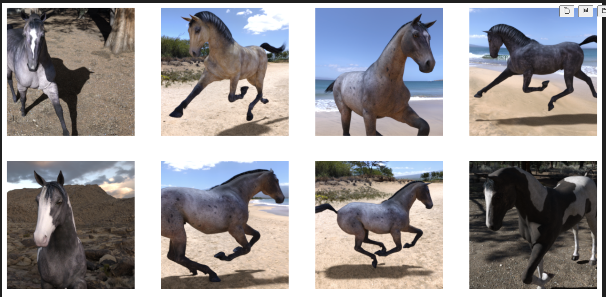
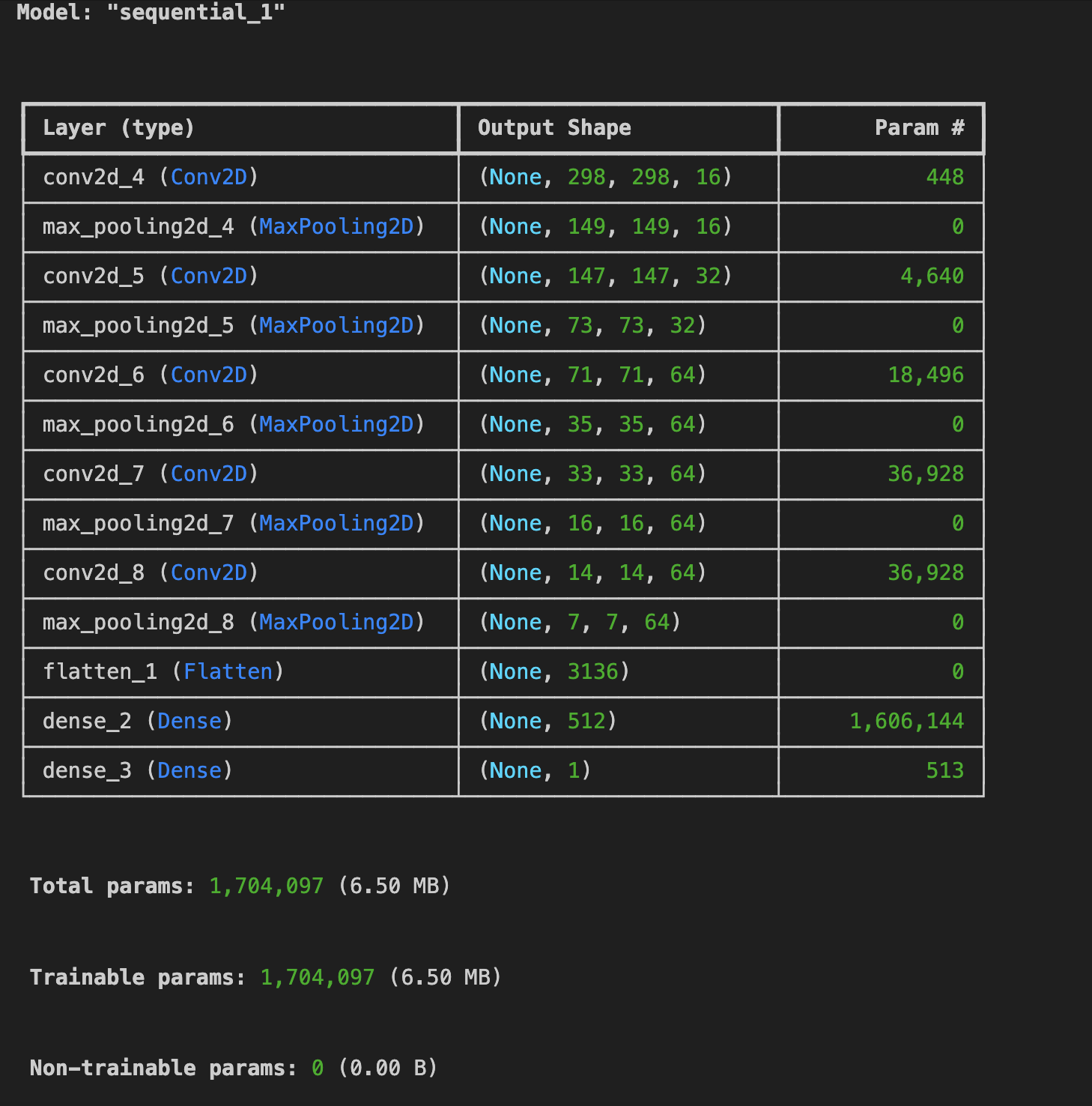
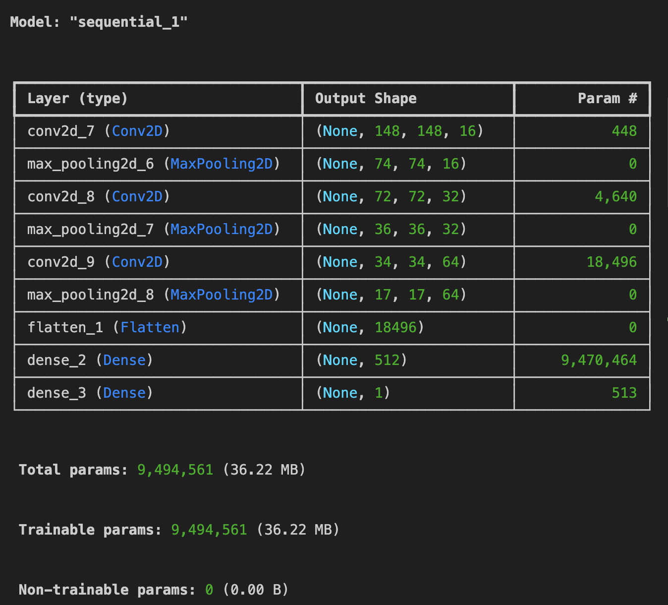
[3] model build
import tensorflow as tf

model = tf.keras.models.Sequential([
    tf.keras.layers.Conv2D(16, (3,3), activation='relu',
                           input_shape=(150,150,3)),
    tf.keras.layers.MaxPooling2D(2,2),
    tf.keras.layers.Conv2D(32, (3,3), activation='relu'),
    tf.keras.layers.MaxPooling2D(2,2),
    tf.keras.layers.Conv2D(64, (3,3), activation='relu'),
    tf.keras.layers.MaxPooling2D(2,2),

    tf.keras.layers.Flatten(),
    tf.keras.layers.Dense(512, activation='relu'),
    tf.keras.layers.Dense(1, activation='sigmoid')
])

model.summary()
input_shape 사이즈가 (300,300)에서 (150,150) 으로 줄었고,
Conv2D 레이어 3개로 쌓았다.
[4] model compile
model.compile(
    loss='binary_crossentropy',
    metrics=['accuracy'],
    optimizer=tf.keras.optimizers.RMSprop(learning_rate=0.001)
)
[5] 학습/검증 ImageGenerator 생성
from tensorflow.keras.preprocessing.image import ImageDataGenerator

train_datagen = ImageDataGenerator(rescale=1/255)
validation_datagen = ImageDataGenerator(rescale=1/255)

train_generator = train_datagen.flow_from_directory(
    './horse-or-human/',
    target_size=(150,150),
    class_mode='binary',
    batch_size = 128
)

validation_generator = validation_datagen.flow_from_directory(
    './validation-horse-or-human/',
    target_size=(150,150),
    class_mode = 'binary',
    batch_size=32,

)

#output

Found 1027 images belonging to 2 classes.
Found 256 images belonging to 2 classes.
기존의 (300,300) 사이즈를 (150,150) 으로 줄였고
검증 데이터의 배치사이즈는 32로 줄였다.
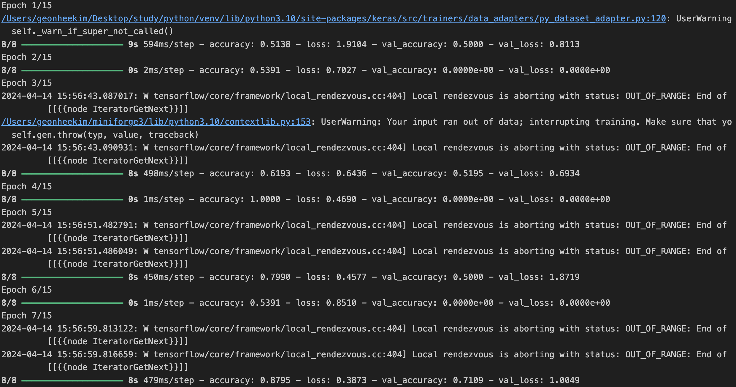
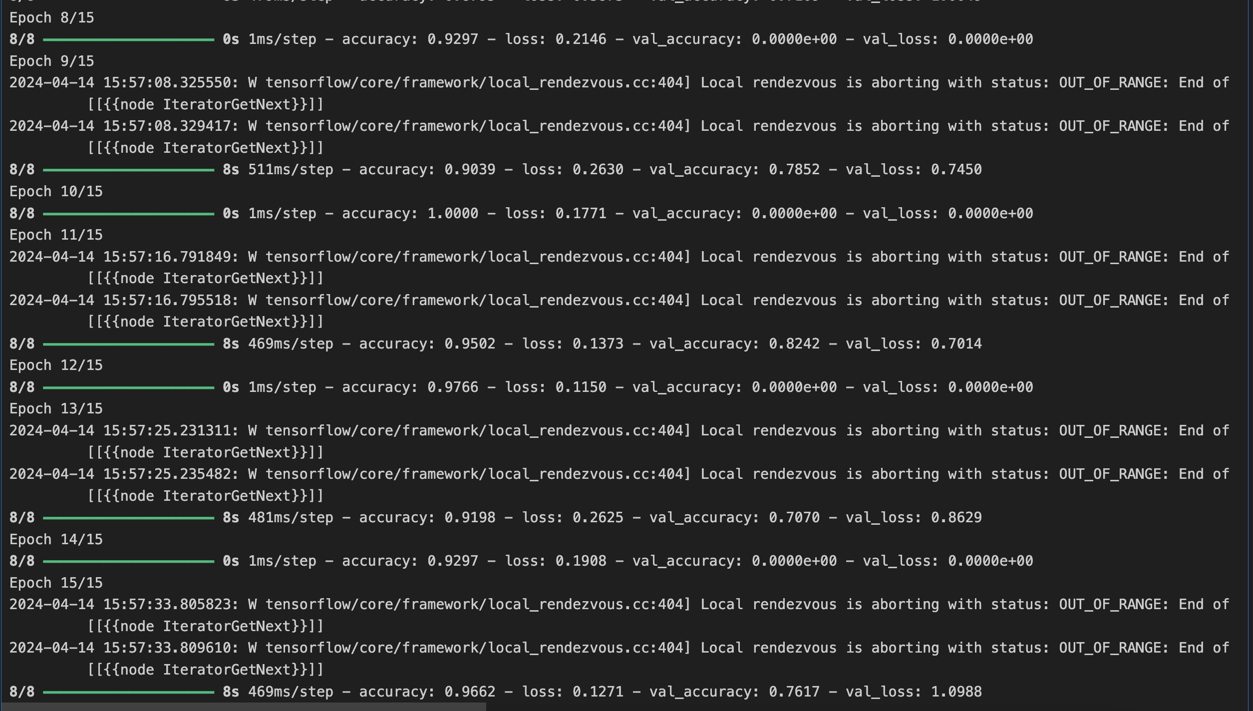
[6] 모델 학습
history = model.fit(
    train_generator,
    steps_per_epoch=8,
    epochs=15,
    validation_data = validation_generator,
    validation_steps=8
)
[7] 모델 예측
import numpy as np
from tensorflow.keras.utils import load_img, img_to_array
path1 = './test_horse.jpg'
path2 = './test_human.jpg'
for path in [path1,path2]:
img = load_img(path, target_size=(150, 150))
x = img_to_array(img)
x /= 255
x = np.expand_dims(x, axis=0)
images = np.vstack([x])
classes = model.predict(images, batch_size=10)
print(classes[0])
if classes[0] > 0.5:
print("The image is predicted to contain a human.")
else:
print("The image is predicted to contain a horse.")
# output
1/1 ━━━━━━━━━━━━━━━━━━━━ 0s 44ms/step
[0.00024391]
The image is predicted to contain a horse.
1/1 ━━━━━━━━━━━━━━━━━━━━ 0s 12ms/step
[0.94135547]
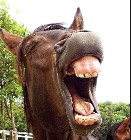
The image is predicted to contain a human.path1 의 이미지
path2 의 이미지

[8] Visualizing Intermediate Representations
%matplotlib inline

import matplotlib.pyplot as plt
import numpy as np
import random
from tensorflow.keras.utils import img_to_array, load_img

# Define a new Model that will take an image as input, and will output
# intermediate representations for all layers in the previous model after
# the first.
successive_outputs = [layer.output for layer in model.layers[1:]]
visualization_model = tf.keras.models.Model(inputs = model.inputs, outputs = successive_outputs)

# Prepare a random input image from the training set.
horse_img_files = [os.path.join(train_horse_dir, f) for f in train_horse_names]
human_img_files = [os.path.join(train_human_dir, f) for f in train_human_names]
img_path = random.choice(horse_img_files + human_img_files)
img = load_img(img_path, target_size=(150, 150))  # this is a PIL image
x = img_to_array(img)  # Numpy array with shape (150, 150, 3)
x = x.reshape((1,) + x.shape)  # Numpy array with shape (1, 150, 150, 3)

# Scale by 1/255
x /= 255

# Run the image through the network, thus obtaining all
# intermediate representations for this image.
successive_feature_maps = visualization_model.predict(x)

# These are the names of the layers, so you can have them as part of the plot
layer_names = [layer.name for layer in model.layers[1:]]

# Display the representations
for layer_name, feature_map in zip(layer_names, successive_feature_maps):
  if len(feature_map.shape) == 4:

    # Just do this for the conv / maxpool layers, not the fully-connected layers
    n_features = feature_map.shape[-1]  # number of features in feature map

    # The feature map has shape (1, size, size, n_features)
    size = feature_map.shape[1]

    # Tile the images in this matrix
    display_grid = np.zeros((size, size * n_features))
    for i in range(n_features):
      x = feature_map[0, :, :, i]
      x -= x.mean()
      x /= x.std()
      x *= 64
      x += 128
      x = np.clip(x, 0, 255).astype('uint8')

      # Tile each filter into this big horizontal grid
      display_grid[:, i * size : (i + 1) * size] = x

    # Display the grid
    scale = 20. / n_features
    plt.figure(figsize=(scale * n_features, scale))
    plt.title(layer_name)
    plt.grid(False)
    plt.imshow(display_grid, aspect='auto', cmap='viridis')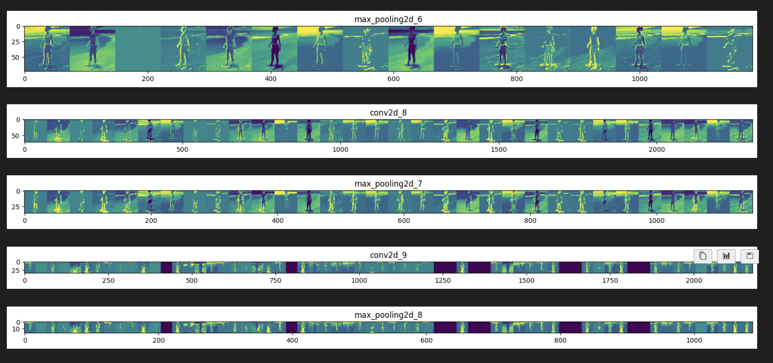

꿈꾸는 것도 개발처럼 깊게