D.I.P. - Final Exam
Q1
% Q1
clear all; close all; clc;

% (128, 128)
% Image_NZP(ver. Non-Zero-Padding)
I_NZP = double(phantom(128));
I_NZP = I_NZP/max(I_NZP(:));
Size_I_NZP = max(size(I_NZP, 1), size(I_NZP, 2));

% Image_NZP Index 좌표(ver. Non-Zero-Padding)
[Ny_NZP, Nx_NZP] = size(I_NZP);
cx_NZP = floor(Nx_NZP/2) + 1; % Image_NZP 중앙 x 인덱스
cy_NZP = floor(Ny_NZP/2) + 1; % Image_NZP 중앙 y 인덱스

% Image_ZP Index 좌표(ver. Zero-Padding)
I_ZP = zeros([256, 256]); % 가로 256줄 세로 256줄
[Ny_ZP, Nx_ZP] = size(I_ZP);
cx_ZP = floor(Nx_ZP/2) + 1; % Image_ZP 중앙 x 인덱스
cy_ZP = floor(Ny_ZP/2) + 1; % Image_ZP 중앙 y 인덱스

% Image_ZP(ver. Zero-Padding)
I_ZP(cy_ZP-Ny_NZP/2+1:cy_ZP+Ny_NZP/2, cx_ZP-Nx_NZP/2+1:cx_ZP+Nx_NZP/2) = I_NZP;
Size_I_ZP = max(size(I_ZP, 1), size(I_ZP, 2));

% 각도 조정
Del_Theta = 1;
Theta = 0:Del_Theta:180-Del_Theta;
num_angles = length(Theta);

% Sinogram 생성
proj1 = zeros(Size_I_NZP, num_angles);
for i = 1:num_angles
    proj1(:,i) = sum(imrotate(I_NZP, -Theta(i), 'bilinear', 'crop'), 1);
end

% Sinogram 생성
proj2 = zeros(Size_I_ZP, num_angles);
for i = 1:num_angles
    proj2(:,i) = sum(imrotate(I_ZP, -Theta(i), 'bilinear', 'crop'), 1);
end

figure;
subplot(1, 2, 1)
imagesc(Theta, 1:Size_I_NZP, proj1);
colormap gray; colorbar;
xlabel('\theta (deg)');
ylabel('Detector index');
title('Sinogram (Non-Zero-Padding)');

subplot(1, 2, 2)
imagesc(Theta, 1:Size_I_ZP, proj2);
colormap gray; colorbar;
xlabel('\theta (deg)');
ylabel('Detector index');
title('Sinogram (Zero-Padding)');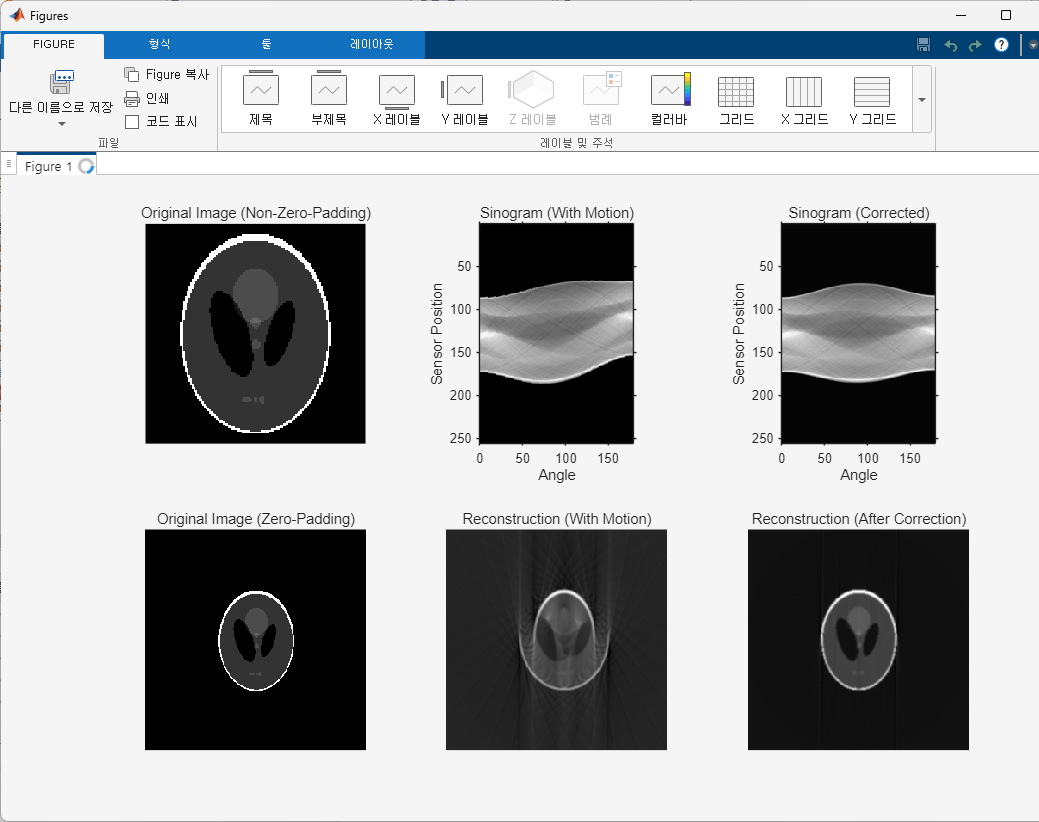
Q2
% Q2
clear all; close all; clc;

% (128 128)
% Image_NZP (ver. Non-Zero-Padding)
I_NZP = double(phantom(128));
I_NZP = I_NZP/max(I_NZP(:));
Size_I_NZP = max(size(I_NZP, 1), size(I_NZP, 2));

% Image_NZP Index 좌표 (ver. Non-Zero-Padding)
[Ny_NZP, Nx_NZP] = size(I_NZP);
cx_NZP = floor(Nx_NZP/2) + 1; % Image_NZP 중앙 x 인덱스
cy_NZP = floor(Ny_NZP/2) + 1; % Image_NZP 중앙 y 인덱스

% Image_ZP Index 좌표 (ver. Zero-Padding)
I_ZP = zeros([256, 256]); % 가로 256줄 세로 256줄
[Ny_ZP, Nx_ZP] = size(I_ZP);
cx_ZP = floor(Nx_ZP/2) + 1; % Image_ZP 중앙 x 인덱스
cy_ZP = floor(Ny_ZP/2) + 1; % Image_ZP 중앙 y 인덱스

% Image_ZP (ver. Zero-Padding)
I_ZP(cy_ZP-Ny_NZP/2+1:cy_ZP+Ny_NZP/2, cx_ZP-Nx_NZP/2+1:cx_ZP+Nx_NZP/2) = I_NZP;
Size_I_ZP = max(size(I_ZP, 1), size(I_ZP, 2));

% 각도 조정
Del_Theta = 1;
Theta = 0:Del_Theta:180-Del_Theta;
num_angles = length(Theta);

% Sinogram 생성 (ver. Non-Zero-Padding)
proj_1 = zeros(Size_I_NZP, num_angles);
for i = 1:num_angles
    proj_1(:,i) = sum(imrotate(I_NZP, -Theta(i), 'bilinear', 'crop'), 1);
end

% Sinogram 생성 (ver. Zero-Padding)
proj_2 = zeros(Size_I_ZP, num_angles);
for i = 1:num_angles
    proj_2(:,i) = sum(imrotate(I_ZP, -Theta(i), 'bilinear', 'crop'), 1);
end

% Non-Zero_Padding Reconstruction
Recon_I_NZP_No_Filter = iradon(proj_1, Theta, 'linear', 'none', Size_I_NZP);
Recon_I_NZP_RamLak = iradon(proj_1, Theta, 'linear', 'ram-lak', Size_I_NZP);
Recon_I_NZP_HammingWindowedRamLak = iradon(proj_1, Theta, 'linear', 'hann', Size_I_NZP);

% Non-Zero-Padding Reconstruction (direct FBP)
Recon_I_NZP_No_Filter_direct = my_fbp(proj_1, Theta, 'none', Size_I_NZP);
Recon_I_NZP_RamLak_direct = my_fbp(proj_1, Theta, 'ram-lak', Size_I_NZP);
Recon_I_NZP_Hann_direct = my_fbp(proj_1, Theta, 'hann', Size_I_NZP);

% Zero-Padding Reconstruction
Recon_I_ZP_No_Filter = iradon(proj_2, Theta, 'none', Size_I_ZP);
Recon_I_ZP_RamLak = iradon(proj_2, Theta, 'ram-lak', Size_I_ZP);
Recon_I_ZP_HammingWindowedRamLak = iradon(proj_2, Theta, 'hann', Size_I_ZP);

% Zero-Padding Reconstruction (direct FBP)
Recon_I_ZP_No_Filter_direct = my_fbp(proj_2, Theta, 'none', Size_I_ZP);
Recon_I_ZP_RamLak_direct = my_fbp(proj_2, Theta, 'ram-lak', Size_I_ZP);
Recon_I_ZP_Hann_direct = my_fbp(proj_2, Theta, 'hann', Size_I_ZP);

% MSE
MSE_NZP_No_Filter = mean((Recon_I_NZP_No_Filter(:) - I_NZP(:)).^2);
MSE_NZP_RamLak = mean((Recon_I_NZP_RamLak(:) - I_NZP(:)).^2);
MSE_NZP_Hann = mean((Recon_I_NZP_HammingWindowedRamLak(:) - I_NZP(:)).^2);

MSE_NZP_No_Filter_direct = mean((Recon_I_NZP_No_Filter_direct(:) - I_NZP(:)).^2);
MSE_NZP_RamLak_direct = mean((Recon_I_NZP_RamLak_direct(:) - I_NZP(:)).^2);
MSE_NZP_Hann_direct = mean((Recon_I_NZP_Hann_direct(:) - I_NZP(:)).^2);

MSE_ZP_No_Filter = mean((Recon_I_ZP_No_Filter(:) - I_ZP(:)).^2);
MSE_ZP_RamLak = mean((Recon_I_ZP_RamLak(:) - I_ZP(:)).^2);
MSE_ZP_Hann = mean((Recon_I_ZP_HammingWindowedRamLak(:) - I_ZP(:)).^2);

MSE_ZP_No_Filter_direct = mean((Recon_I_ZP_No_Filter_direct(:) - I_ZP(:)).^2);
MSE_ZP_RamLak_direct = mean((Recon_I_ZP_RamLak_direct(:) - I_ZP(:)).^2);
MSE_ZP_Hann_direct = mean((Recon_I_ZP_Hann_direct(:) - I_ZP(:)).^2);

figure;

subplot(2, 5, 1);
imshow(I_NZP, []);
title('Image (Non-Zero-Padding)');
subplot(2, 5, 2);
imagesc(Theta, 1:Size_I_NZP, proj_1);
colormap gray; colorbar; xlabel('\theta (deg)'); ylabel('Detector index');
title('Sinogram (Non-Zero-Padding)');
subplot(2, 5, 3);
imshow(Recon_I_NZP_No_Filter_direct, []);
title(sprintf('Reconstruction of Image\nNo Filter without iradon'));
subplot(2, 5, 4);
imshow(Recon_I_NZP_RamLak_direct, []);
title(sprintf('Reconstruction of Image\nRamLak without iradon'));
subplot(2, 5, 5);
imshow(Recon_I_NZP_Hann_direct, []);
title(sprintf('Reconstruction of Image\nHann without iradon'));
subplot(2, 5, 6);
imshow(I_NZP, []);
title('Image (Non-Zero-Padding)');
subplot(2, 5, 7);
imagesc(Theta, 1:Size_I_NZP, proj_1);
colormap gray; colorbar; xlabel('\theta (deg)'); ylabel('Detector index');
title('Sinogram (Non-Zero-Padding)');
subplot(2, 5, 8);
imshow(Recon_I_NZP_No_Filter, []);
title(sprintf('Reconstruction of Image\nNo Filter with iradon'));
subplot(2, 5, 9);
imshow(Recon_I_NZP_RamLak, []);
title(sprintf('Reconstruction of Image\nRamLak with iradon'));
subplot(2, 5, 10);
imshow(Recon_I_NZP_HammingWindowedRamLak, []);
title(sprintf('Reconstruction of Image\nHann with iradon'));

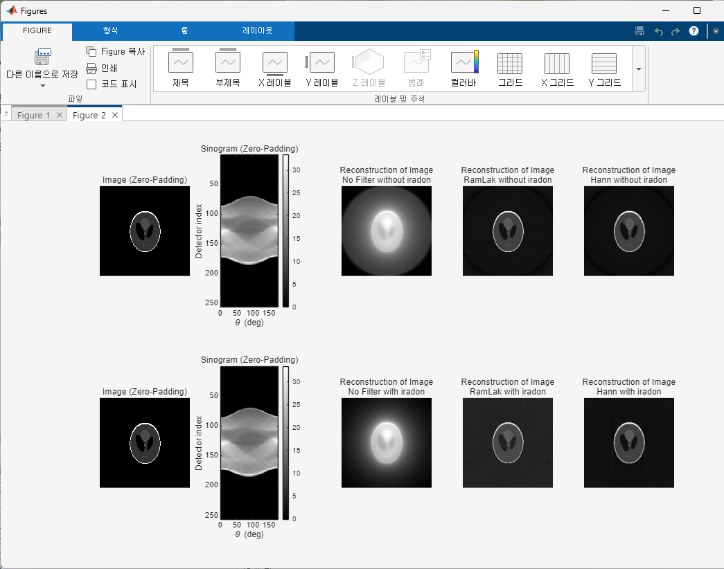
figure;
subplot(2, 5, 1);
imshow(I_ZP, []);
title('Image (Zero-Padding)');
subplot(2, 5, 2);
imagesc(Theta, 1:Size_I_ZP, proj_2);
colormap gray; colorbar; xlabel('\theta (deg)'); ylabel('Detector index');
title('Sinogram (Zero-Padding)');
subplot(2, 5, 3);
imshow(Recon_I_ZP_No_Filter_direct, []);
title(sprintf('Reconstruction of Image\nNo Filter without iradon'));
subplot(2, 5, 4);
imshow(Recon_I_ZP_RamLak_direct, []);
title(sprintf('Reconstruction of Image\nRamLak without iradon'));
subplot(2, 5, 5);
imshow(Recon_I_ZP_Hann_direct, []);
title(sprintf('Reconstruction of Image\nHann without iradon'));
subplot(2, 5, 6);
imshow(I_ZP, []);
title('Image (Zero-Padding)');
subplot(2, 5, 7);
imagesc(Theta, 1:Size_I_ZP, proj_2);
colormap gray; colorbar; xlabel('\theta (deg)'); ylabel('Detector index');
title('Sinogram (Zero-Padding)');
subplot(2, 5, 8);
imshow(Recon_I_ZP_No_Filter, []);
title(sprintf('Reconstruction of Image\nNo Filter with iradon'));
subplot(2, 5, 9);
imshow(Recon_I_ZP_RamLak, []);
title(sprintf('Reconstruction of Image\nRamLak with iradon'));
subplot(2, 5, 10);
imshow(Recon_I_ZP_HammingWindowedRamLak, []);
title(sprintf('Reconstruction of Image\nHann with iradon'));

fprintf("MSE_NZP_No_Filter = %f\n", MSE_NZP_No_Filter);
fprintf("MSE_NZP_RamLak = %f\n", MSE_NZP_RamLak);
fprintf("MSE_NZP_Hann = %f\n", MSE_NZP_Hann);
fprintf("MSE_NZP_No_Filter_direct = %f\n", MSE_NZP_No_Filter_direct);
fprintf("MSE_NZP_RamLak_direct = %f\n", MSE_NZP_RamLak_direct);
fprintf("MSE_NZP_Hann_direct = %f\n", MSE_NZP_Hann_direct);
fprintf("MSE_ZP_No_Filter = %f\n", MSE_ZP_No_Filter);
fprintf("MSE_ZP_RamLak = %f\n", MSE_ZP_RamLak);
fprintf("MSE_ZP_Hann = %f\n", MSE_ZP_Hann);
fprintf("MSE_ZP_No_Filter_direct = %f\n", MSE_ZP_No_Filter_direct);
fprintf("MSE_ZP_RamLak_direct = %f\n", MSE_ZP_RamLak_direct);
fprintf("MSE_ZP_Hann_direct = %f\n", MSE_ZP_Hann_direct);

function img = my_fbp(proj, Theta, filter_type, out_size)
    [N, num_angles] = size(proj);

    % 주파수 필터 만들기
    n = (-N/2 : N/2-1)';
    freq = n / (N/2);

    switch lower(filter_type)
        case 'none'
            H = ones(N,1);
        case 'ram-lak'
            H = abs(freq);    % Ram-Lak
        case 'hann'
            H = abs(freq) .* (0.5 + 0.5*cos(pi*freq)); % Hann windowed Ram-Lak
        otherwise
            error('Unknown filter type: %s', filter_type);
    end

    % sinogram을 주파수 영역에서 필터링
    % FFT (detector 방향: 행 방향)
    P = fftshift(fft(fftshift(proj,1), [], 1), 1);
    % 필터 적용
    P_filtered = P .* H;
    % IFFT
    proj_filtered = real(ifftshift(ifft(ifftshift(P_filtered,1), [], 1),1));
    % Backprojection
    img_bp = zeros(N, N);

    for i = 1:num_angles
        col = proj_filtered(:, i);
        row = col';
        bp_slice = repmat(row, N, 1);
        bp_rot   = imrotate(bp_slice, Theta(i), 'bilinear', 'crop');
        img_bp   = img_bp + bp_rot;
    end
    img_bp = img_bp * (pi / (2 * num_angles));

    if N ~= out_size
        start = floor((N - out_size)/2) + 1;
        img = img_bp(start:start+out_size-1, start:start+out_size-1);
    else
        img = img_bp;
    end
end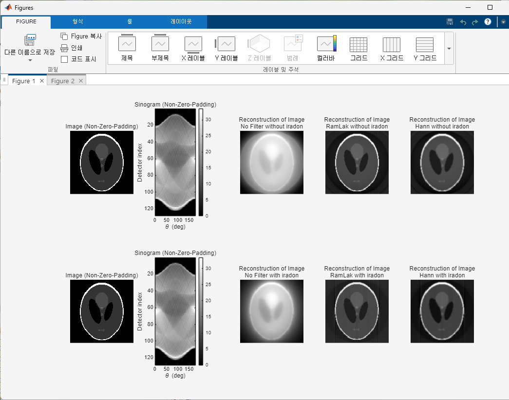
Q3
% Q3
clear all; close all; clc;

% (128 128)
% Image_NZP (ver. Non-Zero-Padding)
I_NZP = double(phantom(128));
I_NZP = I_NZP/max(I_NZP(:));
Size_I_NZP = max(size(I_NZP, 1), size(I_NZP, 2));

% Image_NZP Index 좌표 (ver. Non-Zero-Padding)
[Ny_NZP, Nx_NZP] = size(I_NZP);
cx_NZP = floor(Nx_NZP/2) + 1; % Image_NZP 중앙 x 인덱스
cy_NZP = floor(Ny_NZP/2) + 1; % Image_NZP 중앙 y 인덱스

% Image_NZP + Gaussian Random Noise (mean = 0.2, standard deviation = 0.2)
Gaussian_Random_Noise = 0.2 + 0.2 * randn(size(I_NZP, 1), size(I_NZP, 2));
I_NZP_Noisy = I_NZP + Gaussian_Random_Noise;
Size_I_NZP_Noisy = max(size(I_NZP_Noisy, 1), size(I_NZP_Noisy, 2));

% Image_ZP Index 좌표 (ver. Zero-Padding)
I_ZP = zeros([256, 256]); % 가로 256줄 세로 256줄
[Ny_ZP, Nx_ZP] = size(I_ZP);
cx_ZP = floor(Nx_ZP/2) + 1; % Image_ZP 중앙 x 인덱스
cy_ZP = floor(Ny_ZP/2) + 1; % Image_ZP 중앙 y 인덱스

% Image_ZP (ver. Zero-Padding)
I_ZP(cy_ZP-Ny_NZP/2+1:cy_ZP+Ny_NZP/2, cx_ZP-Nx_NZP/2+1:cx_ZP+Nx_NZP/2) = I_NZP;
Size_I_ZP = max(size(I_ZP, 1), size(I_ZP, 2));

% Image_ZP + Gaussian Random Noise (mean = 0.2, std = 0.2) (ver. Zero-Padding)
I_ZP_Noisy = zeros(size(I_ZP));
I_ZP_Noisy(cy_ZP-Ny_NZP/2+1:cy_ZP+Ny_NZP/2, cx_ZP-Nx_NZP/2+1:cx_ZP+Nx_NZP/2) = I_NZP_Noisy;
Size_I_ZP_Noisy = max(size(I_ZP_Noisy, 1), size(I_ZP_Noisy, 2));

% 각도 조정
Del_Theta = 1;
Theta = 0:Del_Theta:180-Del_Theta;
num_angles = length(Theta);

% Sinogram 생성 (ver. Non-Zero-Padding + Gaussian Random Noise)
proj_2 = zeros(Size_I_NZP_Noisy, num_angles);
for i = 1:num_angles
    proj_2(:,i) = sum(imrotate(I_NZP_Noisy, -Theta(i), 'bilinear', 'crop'), 1);
end

% Sinogram 생성 (ver. Zero-Padding + Gaussian Random Noise)
proj_4 = zeros(Size_I_ZP_Noisy, num_angles);
for i = 1:num_angles
    proj_4(:,i) = sum(imrotate(I_ZP_Noisy, -Theta(i), 'bilinear', 'crop'), 1);
end

% Non-Zero-Padding with Gaussian Random Noise Reconstruction
Recon_I_NZP_Noisy_No_Filter = iradon(proj_2, Theta, 'linear', 'none', Size_I_NZP_Noisy);
Recon_I_NZP_Noisy_RamLak = iradon(proj_2, Theta, 'linear', 'ram-lak', Size_I_NZP_Noisy);
Recon_I_NZP_Noisy_HammingWindowedRamLak = iradon(proj_2, Theta, 'linear', 'hann', Size_I_NZP_Noisy);

% Zero-Padding with Gaussian Random Noise Reconstruction
Recon_I_ZP_Noisy_No_Filter = iradon(proj_4, Theta, 'linear', 'none', Size_I_ZP_Noisy);
Recon_I_ZP_Noisy_RamLak = iradon(proj_4, Theta, 'linear', 'ram-lak', Size_I_ZP_Noisy);
Recon_I_ZP_Noisy_HammingWindowedRamLak = iradon(proj_4, Theta, 'linear', 'hann', Size_I_ZP_Noisy);

% Non-Zero-Padding with Gaussian Random Noise Reconstruction (direct FBP)
Recon_I_NZP_Noisy_No_Filter_direct = my_fbp(proj_2, Theta, 'none', Size_I_NZP_Noisy);
Recon_I_NZP_Noisy_RamLak_direct = my_fbp(proj_2, Theta, 'ram-lak', Size_I_NZP_Noisy);
Recon_I_NZP_Noisy_HammingWindowedRamLak_direct = my_fbp(proj_2, Theta, 'hann', Size_I_NZP_Noisy);

% Zero-Padding with Gaussian Random Noise Reconstruction (direct FBP)
Recon_I_ZP_Noisy_No_Filter_direct = my_fbp(proj_4, Theta, 'none', Size_I_ZP_Noisy);
Recon_I_ZP_Noisy_RamLak_direct = my_fbp(proj_4, Theta, 'ram-lak', Size_I_ZP_Noisy);
Recon_I_ZP_Noisy_HammingWindowedRamLak_direct = my_fbp(proj_4, Theta, 'hann', Size_I_ZP_Noisy);

% MSE
MSE_NZP_Noisy_No_Filter = mean((Recon_I_NZP_Noisy_No_Filter(:) - I_NZP(:)).^2);
MSE_NZP_Noisy_RamLak = mean((Recon_I_NZP_Noisy_RamLak(:) - I_NZP(:)).^2);
MSE_NZP_Noisy_Hann = mean((Recon_I_NZP_Noisy_HammingWindowedRamLak(:) - I_NZP(:)).^2);

MSE_NZP_Noisy_No_Filter_direct = mean((Recon_I_NZP_Noisy_No_Filter_direct(:) - I_NZP(:)).^2);
MSE_NZP_Noisy_RamLak_direct = mean((Recon_I_NZP_Noisy_RamLak_direct(:) - I_NZP(:)).^2);
MSE_NZP_Noisy_Hann_direct = mean((Recon_I_NZP_Noisy_HammingWindowedRamLak_direct(:) - I_NZP(:)).^2);

MSE_ZP_Noisy_No_Filter = mean((Recon_I_ZP_Noisy_No_Filter(:) - I_ZP(:)).^2);
MSE_ZP_Noisy_RamLak = mean((Recon_I_ZP_Noisy_RamLak(:) - I_ZP(:)).^2);
MSE_ZP_Noisy_Hann = mean((Recon_I_ZP_Noisy_HammingWindowedRamLak(:) - I_ZP(:)).^2);

MSE_ZP_Noisy_No_Filter_direct = mean((Recon_I_ZP_Noisy_No_Filter_direct(:) - I_ZP(:)).^2);
MSE_ZP_Noisy_RamLak_direct = mean((Recon_I_ZP_Noisy_RamLak_direct(:) - I_ZP(:)).^2);
MSE_ZP_Noisy_Hann_direct = mean((Recon_I_ZP_Noisy_HammingWindowedRamLak_direct(:) - I_ZP(:)).^2);


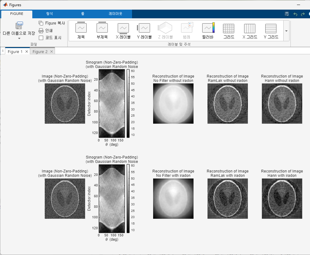
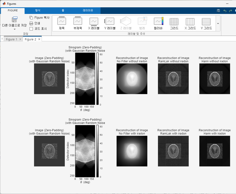
figure;
subplot(2, 5, 1);
imshow(I_NZP_Noisy, []);
title(sprintf('Image (Non-Zero-Padding)\n(with Gaussian Random Noise)'));
subplot(2, 5, 2);
imagesc(Theta, 1:Size_I_NZP, proj_2);
colormap gray; colorbar; xlabel('\theta (deg)'); ylabel('Detector index');
title(sprintf('Sinogram (Non-Zero-Padding)\n(with Gaussian Random Noise'));
subplot(2, 5, 3);
imshow(Recon_I_NZP_Noisy_No_Filter_direct, []);
title(sprintf('Reconstruction of Image\nNo Filter without iradon'));
subplot(2, 5, 4);
imshow(Recon_I_NZP_Noisy_RamLak_direct, []);
title(sprintf('Reconstruction of Image\nRamLak without iradon'));
subplot(2, 5, 5);
imshow(Recon_I_NZP_Noisy_HammingWindowedRamLak_direct, []);
title(sprintf('Reconstruction of Image\nHann without iradon'));
subplot(2, 5, 6);
imshow(I_NZP_Noisy, []);
title(sprintf('Image (Non-Zero-Padding)\n(with Gaussian Random Noise)'));
subplot(2, 5, 7);
imagesc(Theta, 1:Size_I_NZP_Noisy, proj_2);
colormap gray; colorbar; xlabel('\theta (deg)'); ylabel('Detector index');
title(sprintf('Sinogram (Non-Zero-Padding)\n(with Gaussian Random Noise'));
subplot(2, 5, 8);
imshow(Recon_I_NZP_Noisy_No_Filter, []);
title(sprintf('Reconstruction of Image\nNo Filter with iradon'));
subplot(2, 5, 9);
imshow(Recon_I_NZP_Noisy_RamLak, []);
title(sprintf('Reconstruction of Image\nRamLak with iradon'));
subplot(2, 5, 10);
imshow(Recon_I_NZP_Noisy_HammingWindowedRamLak, []);
title(sprintf('Reconstruction of Image\nHann with iradon'));

figure;
subplot(2, 5, 1);
imshow(I_ZP_Noisy, []);
title(sprintf('Image (Zero-Padding)\n(with Gaussian Random Noise)'));
subplot(2, 5, 2);
imagesc(Theta, 1:Size_I_ZP, proj_4);
colormap gray; colorbar; xlabel('\theta (deg)'); ylabel('Detector index');
title(sprintf('Sinogram (Zero-Padding)\n(with Gaussian Random Noise'));
subplot(2, 5, 3);
imshow(Recon_I_ZP_Noisy_No_Filter_direct, []);
title(sprintf('Reconstruction of Image\nNo Filter without iradon'));
subplot(2, 5, 4);
imshow(Recon_I_ZP_Noisy_RamLak_direct, []);
title(sprintf('Reconstruction of Image\nRamLak without iradon'));
subplot(2, 5, 5);
imshow(Recon_I_ZP_Noisy_HammingWindowedRamLak_direct, []);
title(sprintf('Reconstruction of Image\nHann without iradon'));
subplot(2, 5, 6);
imshow(I_ZP_Noisy, []);
title(sprintf('Image (Zero-Padding)\n(with Gaussian Random Noise)'));
subplot(2, 5, 7);
imagesc(Theta, 1:Size_I_ZP_Noisy, proj_4);
colormap gray; colorbar; xlabel('\theta (deg)'); ylabel('Detector index');
title(sprintf('Sinogram (Zero-Padding)\n(with Gaussian Random Noise'));
subplot(2, 5, 8);
imshow(Recon_I_ZP_Noisy_No_Filter, []);
title(sprintf('Reconstruction of Image\nNo Filter with iradon'));
subplot(2, 5, 9);
imshow(Recon_I_ZP_Noisy_RamLak, []);
title(sprintf('Reconstruction of Image\nRamLak with iradon'));
subplot(2, 5, 10);
imshow(Recon_I_ZP_Noisy_HammingWindowedRamLak, []);
title(sprintf('Reconstruction of Image\nHann with iradon'));

fprintf("MSE_NZP_Noisy_No_Filter = %f\n", MSE_NZP_Noisy_No_Filter);
fprintf("MSE_NZP_Noisy_RamLak = %f\n", MSE_NZP_Noisy_RamLak);
fprintf("MSE_NZP_Noisy_Hann = %f\n", MSE_NZP_Noisy_Hann);
fprintf("MSE_NZP_Noisy_No_Filter_direct = %f\n", MSE_NZP_Noisy_No_Filter_direct);
fprintf("MSE_NZP_Noisy_RamLak_direct = %f\n", MSE_NZP_Noisy_RamLak_direct);
fprintf("MSE_NZP_Noisy_Hann_direct = %f\n", MSE_NZP_Noisy_Hann_direct);
fprintf("MSE_ZP_Noisy_No_Filter = %f\n", MSE_ZP_Noisy_No_Filter);
fprintf("MSE_ZP_Noisy_RamLak = %f\n", MSE_ZP_Noisy_RamLak);
fprintf("MSE_ZP_Noisy_Hann = %f\n", MSE_ZP_Noisy_Hann);
fprintf("MSE_ZP_Noisy_No_Filter_direct = %f\n", MSE_ZP_Noisy_No_Filter_direct);
fprintf("MSE_ZP_Noisy_RamLak_direct = %f\n", MSE_ZP_Noisy_RamLak_direct);
fprintf("MSE_ZP_Noisy_Hann_direct = %f\n", MSE_ZP_Noisy_Hann_direct);

function img = my_fbp(proj, Theta, filter_type, out_size)
    [N, num_angles] = size(proj);

    % 주파수 필터 만들기
    n = (-N/2 : N/2-1)';
    freq = n / (N/2);

    switch lower(filter_type)
        case 'none'
            H = ones(N,1);
        case 'ram-lak'
            H = abs(freq);    % Ram-Lak
        case 'hann'
            H = abs(freq) .* (0.5 + 0.5*cos(pi*freq)); % Hann windowed Ram-Lak
        otherwise
            error('Unknown filter type: %s', filter_type);
    end

    % sinogram을 주파수 영역에서 필터링
    % FFT (detector 방향: 행 방향)
    P = fftshift(fft(fftshift(proj,1), [], 1), 1);

    % 필터 적용
    P_filtered = P .* H;

    % IFFT
    proj_filtered = real(ifftshift(ifft(ifftshift(P_filtered,1), [], 1),1));

    % Backprojection
    img_bp = zeros(N, N);

    for i = 1:num_angles
        col = proj_filtered(:, i);
        row = col';
        bp_slice = repmat(row, N, 1);
        bp_rot   = imrotate(bp_slice, Theta(i), 'bilinear', 'crop');
        img_bp   = img_bp + bp_rot;
    end

    img_bp = img_bp * (pi / (2 * num_angles));

    if N ~= out_size
        start = floor((N - out_size)/2) + 1;
        img = img_bp(start:start+out_size-1, start:start+out_size-1);
    else
        img = img_bp;
    end
end
Q4
% Q4
clear all; close all; clc;

% (128 128)
% Image_NZP (ver. Non-Zero-Padding)
I_NZP = double(phantom(128));
I_NZP = I_NZP/max(I_NZP(:));
Size_I_NZP = max(size(I_NZP, 1), size(I_NZP, 2));

% Image_NZP Index 좌표 (ver. Non-Zero-Padding)
[Ny_NZP, Nx_NZP] = size(I_NZP);
cx_NZP = floor(Nx_NZP/2) + 1; % Image_NZP 중앙 x 인덱스
cy_NZP = floor(Ny_NZP/2) + 1; % Image_NZP 중앙 y 인덱스

% Image_NZP + Gaussian Random Noise (mean = 0.2, standard deviation = 0.2)
Gaussian_Random_Noise = 0.2 + 0.2 * randn(size(I_NZP, 1), size(I_NZP, 2));
I_NZP_Noisy = I_NZP + Gaussian_Random_Noise;
Size_I_NZP_Noisy = max(size(I_NZP_Noisy, 1), size(I_NZP_Noisy, 2));

% Image_ZP Index 좌표 (ver. Zero-Padding)
I_ZP = zeros([256, 256]); % 가로 256줄 세로 256줄
[Ny_ZP, Nx_ZP] = size(I_ZP);
cx_ZP = floor(Nx_ZP/2) + 1; % Image_ZP 중앙 x 인덱스
cy_ZP = floor(Ny_ZP/2) + 1; % Image_ZP 중앙 y 인덱스

% Image_ZP (ver. Zero-Padding)
I_ZP(cy_ZP-Ny_NZP/2+1:cy_ZP+Ny_NZP/2, cx_ZP-Nx_NZP/2+1:cx_ZP+Nx_NZP/2) = I_NZP;
Size_I_ZP = max(size(I_ZP, 1), size(I_ZP, 2));

% Image_ZP + Gaussian Random Noise (mean = 0.2, std = 0.2) (ver. Zero-Padding)
I_ZP_Noisy = zeros(size(I_ZP));
I_ZP_Noisy(cy_ZP-Ny_NZP/2+1:cy_ZP+Ny_NZP/2, cx_ZP-Nx_NZP/2+1:cx_ZP+Nx_NZP/2) = I_NZP_Noisy;
Size_I_ZP_Noisy = max(size(I_ZP_Noisy, 1), size(I_ZP_Noisy, 2));

% 각도 조정
Del_Theta_Set = {1, 5, 10, 20};
for k=1:length(Del_Theta_Set)
    Del_Theta = Del_Theta_Set{k};
    Theta = 0:Del_Theta:180-Del_Theta;
    num_angles = length(Theta);

    % Sinogram 생성 (ver. Non-Zero-Padding)
    proj_1 = zeros(Size_I_NZP, num_angles);
    for i = 1:num_angles
        proj_1(:,i) = sum(imrotate(I_NZP, -Theta(i), 'bilinear', 'crop'), 1);
    end

    % Sinogram 생성 (ver. Non-Zero-Padding + Gaussian Random Noise)
    proj_2 = zeros(Size_I_NZP_Noisy, num_angles);
    for i = 1:num_angles
        proj_2(:,i) = sum(imrotate(I_NZP_Noisy, -Theta(i), 'bilinear', 'crop'), 1);
    end

    % Sinogram 생성 (ver. Zero-Padding)
    proj_3 = zeros(Size_I_ZP, num_angles);
    for i = 1:num_angles
        proj_3(:,i) = sum(imrotate(I_ZP, -Theta(i), 'bilinear', 'crop'), 1);
    end

    % Sinogram 생성 (ver. Zero-Padding + Gaussian Random Noise)
    proj_4 = zeros(Size_I_ZP_Noisy, num_angles);
    for i = 1:num_angles
        proj_4(:,i) = sum(imrotate(I_ZP_Noisy, -Theta(i), 'bilinear', 'crop'), 1);
    end

    % Non-Zero_Padding Reconstruction
    Recon_I_NZP_No_Filter = iradon(proj_1, Theta, 'linear', 'none', Size_I_NZP);
    Recon_I_NZP_RamLak = iradon(proj_1, Theta, 'linear', 'ram-lak', Size_I_NZP);
    Recon_I_NZP_HammingWindowedRamLak = iradon(proj_1, Theta, 'linear', 'hann', Size_I_NZP);

    % Non-Zero-Padding with Gaussian Random Noise Reconstruction
    Recon_I_NZP_Noisy_No_Filter = iradon(proj_2, Theta, 'linear', 'none', Size_I_NZP_Noisy);
    Recon_I_NZP_Noisy_RamLak = iradon(proj_2, Theta, 'linear', 'ram-lak', Size_I_NZP_Noisy);
    Recon_I_NZP_Noisy_HammingWindowedRamLak = iradon(proj_2, Theta, 'linear', 'hann', Size_I_NZP_Noisy);

    % Zero-Padding Reconstruction
    Recon_I_ZP_No_Filter = iradon(proj_3, Theta, 'linear', 'none', Size_I_ZP);
    Recon_I_ZP_RamLak = iradon(proj_3, Theta, 'linear', 'ram-lak', Size_I_ZP);
    Recon_I_ZP_HammingWindowedRamLak = iradon(proj_3, Theta, 'linear', 'hann', Size_I_ZP);

    % Zero-Padding with Gaussian Random Noise Reconstruction
    Recon_I_ZP_Noisy_No_Filter = iradon(proj_4, Theta, 'linear', 'none', Size_I_ZP_Noisy);
    Recon_I_ZP_Noisy_RamLak = iradon(proj_4, Theta, 'linear', 'ram-lak', Size_I_ZP_Noisy);
    Recon_I_ZP_Noisy_HammingWindowedRamLak = iradon(proj_4, Theta, 'linear', 'hann', Size_I_ZP_Noisy);

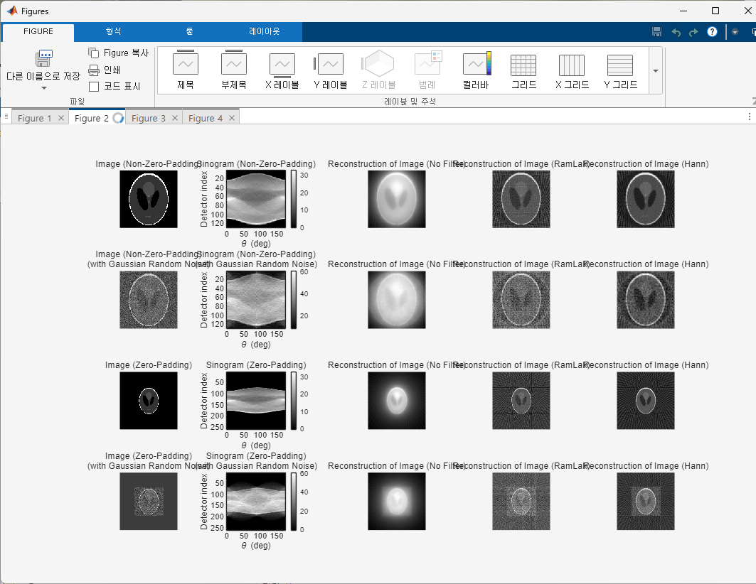
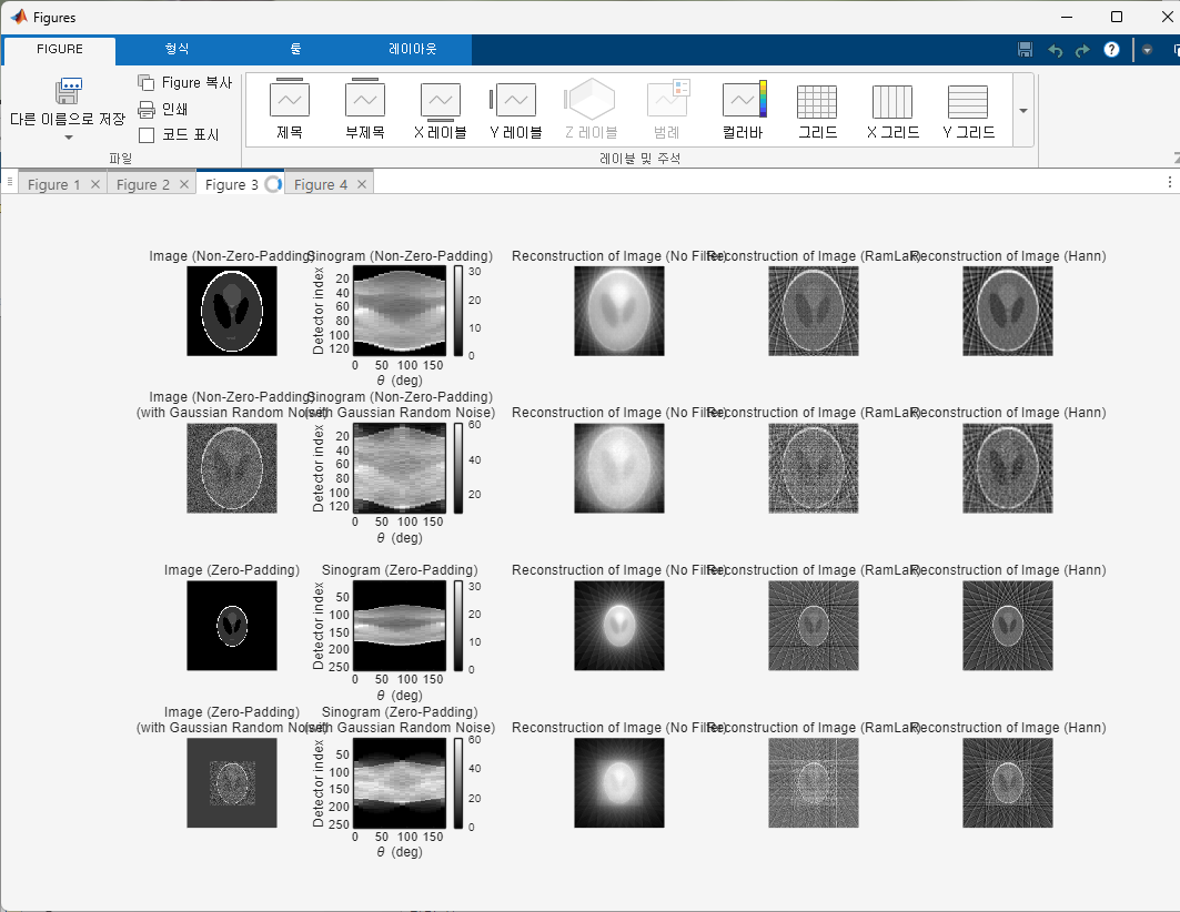
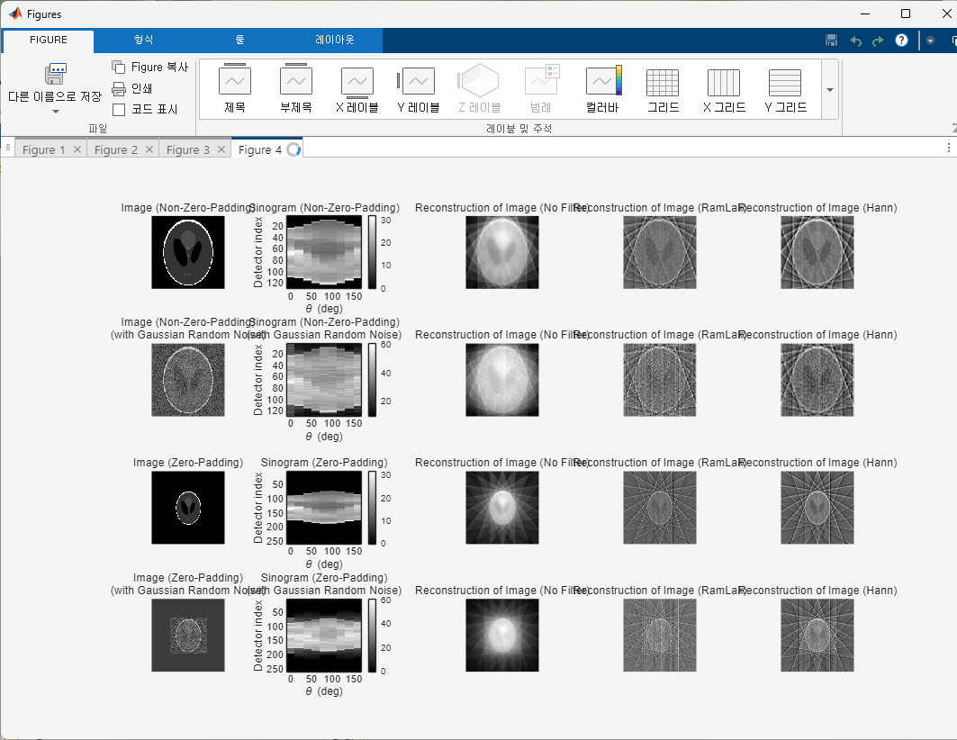
    figure;
    subplot(4, 5, 1);
    imshow(I_NZP, []);
    title('Image (Non-Zero-Padding)');
    subplot(4, 5, 2);
    imagesc(Theta, 1:Size_I_NZP, proj_1);
    colormap gray; colorbar; xlabel('\theta (deg)'); ylabel('Detector index');
    title('Sinogram (Non-Zero-Padding)');
    subplot(4, 5, 3);
    imshow(Recon_I_NZP_No_Filter, []);
    title('Reconstruction of Image (No Filter)');
    subplot(4, 5, 4);
    imshow(Recon_I_NZP_RamLak, []);
    title('Reconstruction of Image (RamLak)');
    subplot(4, 5, 5);
    imshow(Recon_I_NZP_HammingWindowedRamLak, []);
    title('Reconstruction of Image (Hann)');
    subplot(4, 5, 6);
    imshow(I_NZP_Noisy, []);
    title(sprintf('Image (Non-Zero-Padding)\n(with Gaussian Random Noise)'));
    subplot(4, 5, 7);
    imagesc(Theta, 1:Size_I_NZP_Noisy, proj_2);
    colormap gray; colorbar; xlabel('\theta (deg)'); ylabel('Detector index');
    title(sprintf('Sinogram (Non-Zero-Padding)\n(with Gaussian Random Noise)'));
    subplot(4, 5, 8);
    imshow(Recon_I_NZP_Noisy_No_Filter, []);
    title('Reconstruction of Image (No Filter)');
    subplot(4, 5, 9);
    imshow(Recon_I_NZP_Noisy_RamLak, []);
    title('Reconstruction of Image (RamLak)');
    subplot(4, 5, 10);
    imshow(Recon_I_NZP_Noisy_HammingWindowedRamLak, []);
    title('Reconstruction of Image (Hann)');
    subplot(4, 5, 11);
    imshow(I_ZP, []);
    title('Image (Zero-Padding)');
    subplot(4, 5, 12);
    imagesc(Theta, 1:Size_I_ZP, proj_3);
    colormap gray; colorbar; xlabel('\theta (deg)'); ylabel('Detector index');
    title('Sinogram (Zero-Padding)');
    subplot(4, 5, 13);
    imshow(Recon_I_ZP_No_Filter, []);
    title('Reconstruction of Image (No Filter)');
    subplot(4, 5, 14);
    imshow(Recon_I_ZP_RamLak, []);
    title('Reconstruction of Image (RamLak)');
    subplot(4, 5, 15);
    imshow(Recon_I_ZP_HammingWindowedRamLak, []);
    title('Reconstruction of Image (Hann)');
    subplot(4, 5, 16);
    imshow(I_ZP_Noisy, []);
    title(sprintf('Image (Zero-Padding)\n(with Gaussian Random Noise)'));
    subplot(4, 5, 17);
    imagesc(Theta, 1:Size_I_ZP_Noisy, proj_4);
    colormap gray; colorbar; xlabel('\theta (deg)'); ylabel('Detector index');
    title(sprintf('Sinogram (Zero-Padding)\n(with Gaussian Random Noise)'));
    subplot(4, 5, 18);
    imshow(Recon_I_ZP_Noisy_No_Filter, []);
    title('Reconstruction of Image (No Filter)');
    subplot(4, 5, 19);
    imshow(Recon_I_ZP_Noisy_RamLak, []);
    title('Reconstruction of Image (RamLak)');
    subplot(4, 5, 20);
    imshow(Recon_I_ZP_Noisy_HammingWindowedRamLak, []);
    title('Reconstruction of Image (Hann)');
end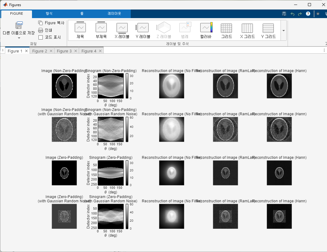
Q5
% Q5
clear all; close all; clc;

% (128 128)
% Image_NZP (ver. Non-Zero-Padding)
I_NZP = double(phantom(128));
I_NZP = I_NZP/max(I_NZP(:));
Size_I_NZP = max(size(I_NZP, 1), size(I_NZP, 2));

% Image_NZP Index 좌표 (ver. Non-Zero-Padding)
[Ny_NZP, Nx_NZP] = size(I_NZP);
cx_NZP = floor(Nx_NZP/2) + 1; % Image_NZP 중앙 x 인덱스
cy_NZP = floor(Ny_NZP/2) + 1; % Image_NZP 중앙 y 인덱스

% Image_ZP Index 좌표 (ver. Zero-Padding)
I_ZP = zeros([256, 256]); % 가로 256줄 세로 256줄
[Ny_ZP, Nx_ZP] = size(I_ZP);
cx_ZP = floor(Nx_ZP/2) + 1; % Image_ZP 중앙 x 인덱스
cy_ZP = floor(Ny_ZP/2) + 1; % Image_ZP 중앙 y 인덱스

% Image_ZP (ver. Zero-Padding)
I_ZP(cy_ZP-Ny_NZP/2+1:cy_ZP+Ny_NZP/2, cx_ZP-Nx_NZP/2+1:cx_ZP+Nx_NZP/2) = I_NZP;
Size_I_ZP = max(size(I_ZP, 1), size(I_ZP, 2));

% 각도 조정
Del_Theta_Set = {0.1, 0.2, 0.5, 1, 2, 5, 10, 20};
for k=1:length(Del_Theta_Set)
    Del_Theta = Del_Theta_Set{k};
    Theta = 0:Del_Theta:180-Del_Theta;
    num_angles = length(Theta);

    % Sinogram 생성 (ver. Non-Zero-Padding)
    proj_1 = zeros(Size_I_NZP, num_angles);
    for i = 1:num_angles
        proj_1(:,i) = sum(imrotate(I_NZP, -Theta(i), 'bilinear', 'crop'), 1);
    end

    % Sinogram 생성 (ver. Zero-Padding)
    proj_3 = zeros(Size_I_ZP, num_angles);
    for i = 1:num_angles
        proj_3(:,i) = sum(imrotate(I_ZP, -Theta(i), 'bilinear', 'crop'), 1);
    end

    % Non-Zero_Padding Reconstruction
    Recon_I_NZP_No_Filter = iradon(proj_1, Theta, 'linear', 'none', Size_I_NZP);
    Recon_I_NZP_RamLak = iradon(proj_1, Theta, 'linear', 'ram-lak', Size_I_NZP);
    Recon_I_NZP_HammingWindowedRamLak = iradon(proj_1, Theta, 'linear', 'hann', Size_I_NZP);

    % Zero-Padding Reconstruction
    Recon_I_ZP_No_Filter = iradon(proj_3, Theta, 'linear', 'none', Size_I_ZP);
    Recon_I_ZP_RamLak = iradon(proj_3, Theta, 'linear', 'ram-lak', Size_I_ZP);
    Recon_I_ZP_HammingWindowedRamLak = iradon(proj_3, Theta, 'linear', 'hann', Size_I_ZP);

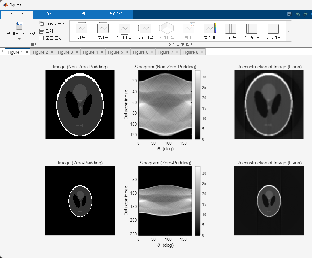
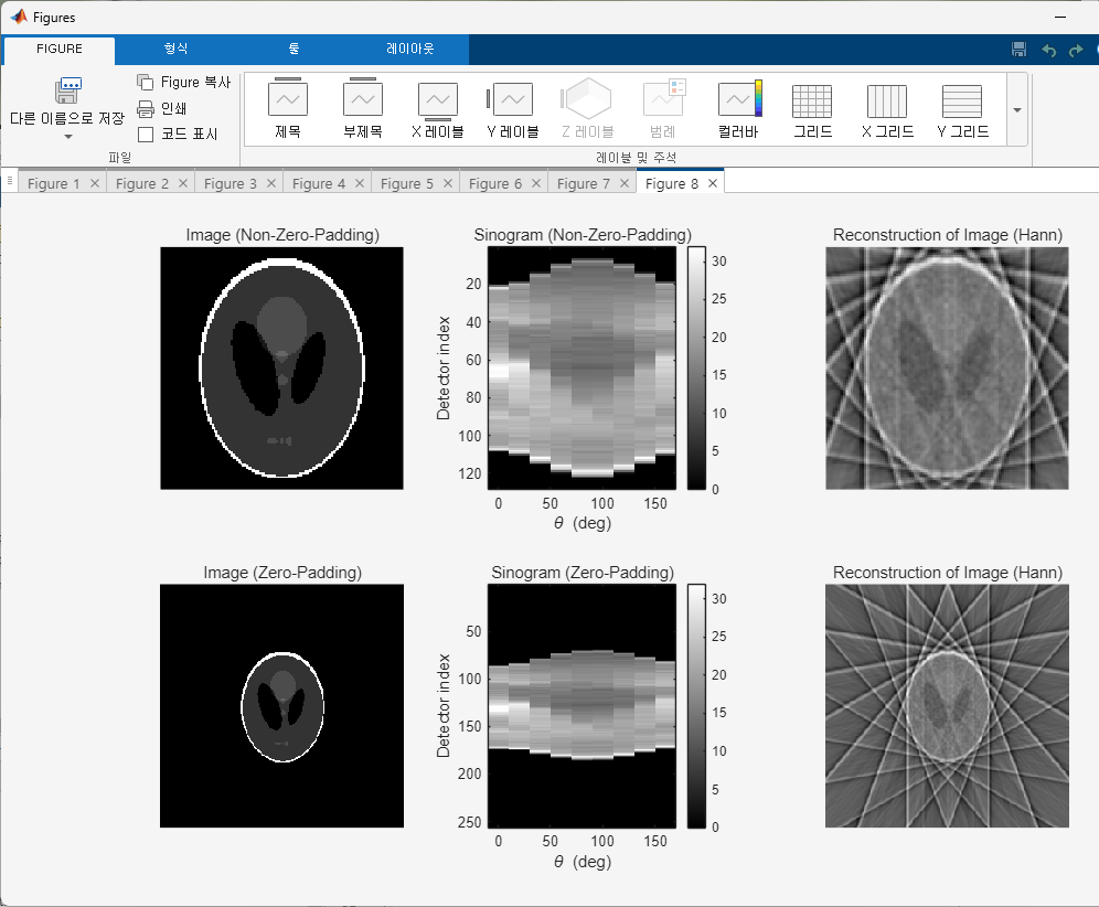
    figure;
    subplot(2, 3, 1);
    imshow(I_NZP, []);
    title('Image (Non-Zero-Padding)');
    subplot(2, 3, 2);
    imagesc(Theta, 1:Size_I_NZP, proj_1);
    colormap gray; colorbar; xlabel('\theta (deg)'); ylabel('Detector index');
    title('Sinogram (Non-Zero-Padding)');
    subplot(2, 3, 3);
    imshow(Recon_I_NZP_HammingWindowedRamLak, []);
    title('Reconstruction of Image (Hann)');
    subplot(2, 3, 4);
    imshow(I_ZP, []);
    title('Image (Zero-Padding)');
    subplot(2, 3, 5);
    imagesc(Theta, 1:Size_I_ZP, proj_3);
    colormap gray; colorbar; xlabel('\theta (deg)'); ylabel('Detector index');
    title('Sinogram (Zero-Padding)');
    subplot(2, 3, 6);
    imshow(Recon_I_ZP_HammingWindowedRamLak, []);
    title('Reconstruction of Image (Hann)');
end
Q6
% Q6
clear all; close all; clc;

% (128 128)
% Image_NZP (ver. Non-Zero-Padding)
I_NZP = double(phantom(128));
I_NZP = I_NZP/max(I_NZP(:));
Size_I_NZP = max(size(I_NZP, 1), size(I_NZP, 2));

% Image_NZP Index 좌표 (ver. Non-Zero-Padding)
[Ny_NZP, Nx_NZP] = size(I_NZP);
cx_NZP = floor(Nx_NZP/2) + 1; % Image_NZP 중앙 x 인덱스
cy_NZP = floor(Ny_NZP/2) + 1; % Image_NZP 중앙 y 인덱스

% Image_ZP Index 좌표 (ver. Zero-Padding)
I_ZP = zeros([256, 256]); % 가로 256줄 세로 256줄
[Ny_ZP, Nx_ZP] = size(I_ZP);
cx_ZP = floor(Nx_ZP/2) + 1; % Image_ZP 중앙 x 인덱스
cy_ZP = floor(Ny_ZP/2) + 1; % Image_ZP 중앙 y 인덱스

% Image_ZP (ver. Zero-Padding)
I_ZP(cy_ZP-Ny_NZP/2+1:cy_ZP+Ny_NZP/2, cx_ZP-Nx_NZP/2+1:cx_ZP+Nx_NZP/2) = I_NZP;
Size_I_ZP = max(size(I_ZP, 1), size(I_ZP, 2));

% Image_ZP + Horizontally Shift (ver. Zero-Padding) (Initial)
I_ZP_H_Shift = I_ZP;
Size_I_ZP_H_Shift = max(size(I_ZP_H_Shift, 1), size(I_ZP_H_Shift, 2));

% 각도 조정
Del_Theta = 1;
Theta = 0:Del_Theta:180-Del_Theta;
num_angles = length(Theta);

% 보정되지 않은 Sinogram, 초기화
proj = zeros(Size_I_ZP_H_Shift, num_angles);
total_shift_amount = 0;

% 보정되지 않은 Sinogram
for i=1:num_angles
    if i > 1 && mod(i-1, 10) == 0
        I_ZP_H_Shift = circshift(I_ZP_H_Shift, [0, 1]);
        total_shift_amount = total_shift_amount + 1;
    end
    proj(:,i) = sum(imrotate(I_ZP_H_Shift, -Theta(i), 'bilinear', 'crop'), 1);
end

% 보정된 Sinogram, 초기화
proj_corrected = zeros(size(proj));
total_shift_amount_corrected = 0;

N = Size_I_ZP;
k = -N/2 : N/2-1;
freqs = (k / N)';

for j = 1:num_angles
    if j > 1 && mod(j-1, 10) == 0
        total_shift_amount_corrected = total_shift_amount_corrected + 1;
    end

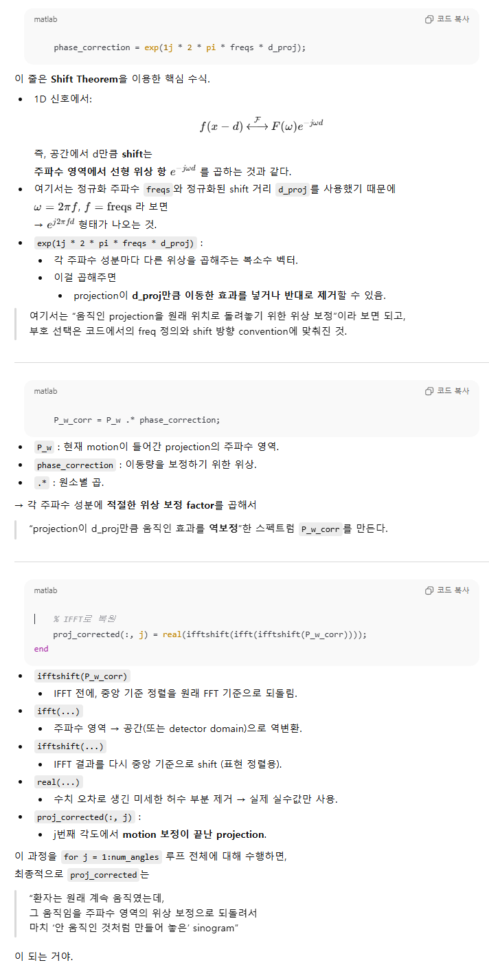
    P_w = fftshift(fft(fftshift(proj(:, j))));

    % 보정
    d_proj = total_shift_amount_corrected * cos(deg2rad(Theta(j)));
    phase_correction = exp(1j * 2 * pi * freqs * d_proj);
    P_w_corr = P_w .* phase_correction;

    % IFFT로 복원
    proj_corrected(:, j) = real(ifftshift(ifft(ifftshift(P_w_corr))));
end


Recon_Motion = iradon(proj, Theta, 'hann', Size_I_ZP);
Recon_Corrected = iradon(proj_corrected, Theta, 'hann', Size_I_ZP);

figure;
subplot(2, 3, 1);
imshow(I_NZP, []); title('Original Image (Non-Zero-Padding)')
subplot(2, 3, 2);
imshow(proj, [], 'XData', Theta, 'YData', 1:Size_I_ZP);
title('Sinogram (With Motion)'); xlabel('Angle'); ylabel('Sensor Position');
axis on;
subplot(2, 3, 3);
imshow(proj_corrected, [], 'XData', Theta, 'YData', 1:Size_I_ZP);
title('Sinogram (Corrected)'); xlabel('Angle'); ylabel('Sensor Position');
axis on;
subplot(2, 3, 4);
imshow(I_ZP, []); title('Original Image (Zero-Padding)');
subplot(2, 3, 5);
imshow(Recon_Motion, []);
title('Reconstruction (With Motion)');
subplot(2, 3, 6);
imshow(Recon_Corrected, []);
title('Reconstruction (After Correction)');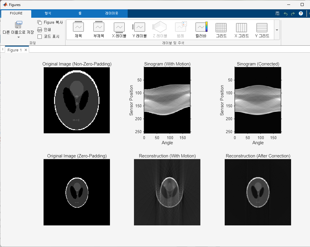
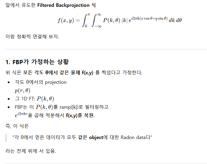
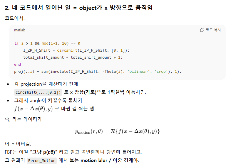
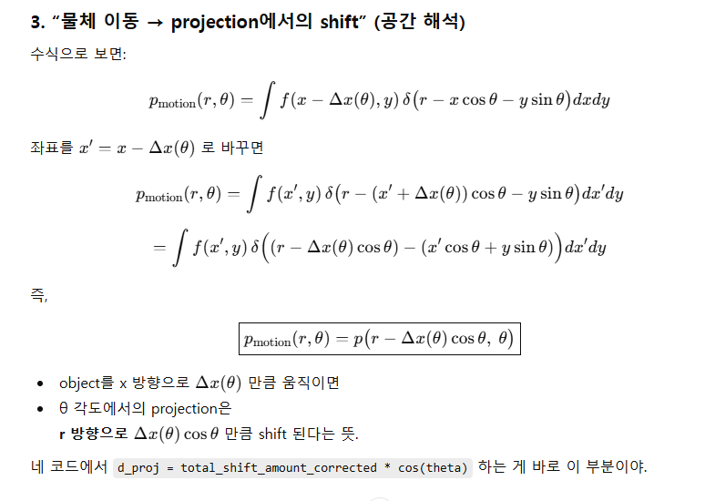
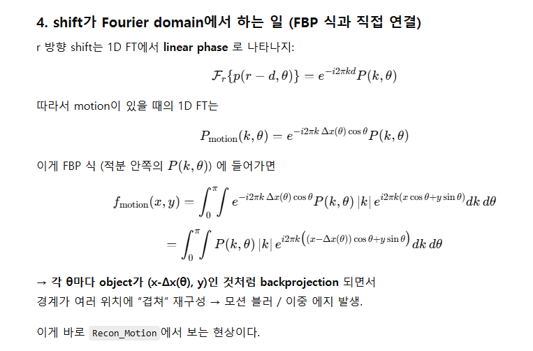
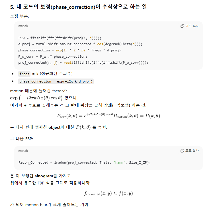
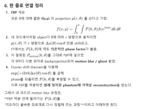
MRI
% % %% 1. 데이터 로드 및 정규화
% % % brain_8ch.mat 안에
% % %   im  : coil image (복소수),  [Nx, Ny, Ns, Nc] 형태라고 가정
% % %   map : sensitivity map,      [Nx, Ny, Ns, Nc]
% % load('brain_8ch.mat');    % im, map
% %
% % % 한 슬라이스만 사용 (3번째 차원: slice)
% % im  = squeeze(im(:,:,:,:));    % [Nx, Ny, Nc]
% % map = squeeze(map(:,:,:,:));   % [Nx, Ny, Nc]
% %
% % % 정규화 (보기 편하게)
% % im  = im  / max(abs(im(:)));
% % map = map / max(abs(map(:)));
% %
% % %% 1-1. Coil image / sensitivity map 확인
% % figure;
% % montage(permute(abs(im), [1, 2, 4, 3]));
% % title('Coil images (magnitude)');
% %
% % figure;
% % montage(permute(abs(map), [1, 2, 4, 3]));
% % title('Sensitivity maps (magnitude)');
% %
% %
% % %% 2. k-space로 변환 후 undersampling (R = 2, 크기는 유지)
% % R = 2;
% %
% % [Nx, Ny, Nc] = size(im);
% %
% % k = fft2(fftshift(im));    % 각 coil에 대해 2D FFT → [Nx, Ny, Nc]
% %
% % % undersampled k-space (라인은 R배 건너뛰고, 나머지는 0으로)
% % k_us = zeros(size(k));        % [Nx, Ny, Nc]
% % k_us(2:R:end, :, :) = k(2:R:end, :, :);
% %
% % % alias 된 coil image (크기는 여전히 [Nx, Ny, Nc])
% % im_us = ifftshift(ifft2(k_us));
% %
% % figure;
% % montage(permute(abs(im_us), [1, 2, 4, 3]));
% % title('Aliased coil images (R = 2)');
% %
% % %% 3. SENSE 복원 - (A''A)^(-1) A'' b 형태 사용
% % sep = Nx / R;                 % 서로 겹치는 두 픽셀 사이 간격 (R=2 → Nx/2)
% %
% % im_sense = zeros(Nx, Ny);     % 복원된 단일 이미지 (complex)
% %
% % for ix = 1:Nx
% %     % 이 alias 픽셀에 겹쳐진 실제 위치 인덱스들 (wrap-around 포함)
% %     orig_idx = ix + (0:R-1) * sep;     % [ix, ix+sep]
% %     orig_idx(orig_idx > Nx) = orig_idx(orig_idx > Nx) - Nx;  % modulo Nx
% %
% %     for iy = 1:Ny
% %         % b : 각 coil에서 측정된 alias 값 F_i  (Nc x 1)
% %         b = squeeze(im_us(ix, iy, :));           % [Nc, 1]
% %
% %         % A : coil sensitivity matrix  (Nc x R)
% %         A = zeros(Nc, R);
% %         for r = 1:R
% %             A(:, r) = squeeze(map(orig_idx(r), iy, :));   % [Nc, 1]
% %         end
% %
% %         % 슬라이드 식: sol = pinv(A' * A) * A' * b
% %         % sol = [I_A; I_B]  (겹치기 전 두 픽셀 값)
% %         sol = pinv(A' * A) * (A' * b);          % [R, 1]
% %
% %         % 복원된 두 픽셀 값을 각 위치에 채워 넣기
% %         im_sense(orig_idx, iy) = sol;
% %     end
% % end
% %
% % %% 4. 결과 표시
% % figure;
% % imshow(abs(im_sense), []);
% % title('SENSE reconstructed image (R = 2, (A^T A)^{-1} A^T b)');
%
%

%% 1. 데이터 로드 및 정규화
load('brain_8ch.mat');    % im: coil images, map: coil sensitivity

% 한 슬라이스만 사용한다고 가정 (필요하면 (:,:,1,:) 로 바꿔도 됨)
im  = squeeze(im(:,:,:,:));   % [Nx, Ny, Nc]
map = squeeze(map(:,:,:,:));  % [Nx, Ny, Nc]

% 정규화
im  = im  / max(abs(im(:)));
map = map / max(abs(map(:)));

% Coil / map 확인 (하단 코드 스타일 유지)
figure;
montage(permute(abs(im),  [1, 2, 4, 3]));
title('Coil images');

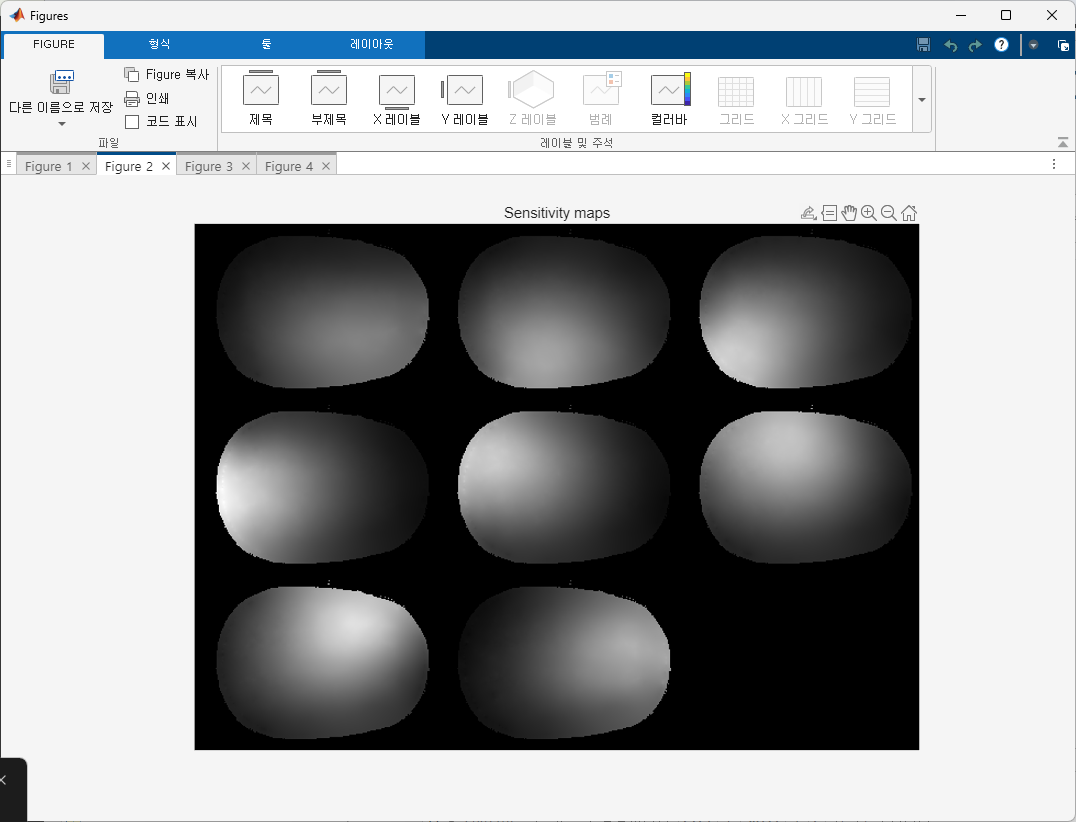
figure;
montage(permute(abs(map), [1, 2, 4, 3]));
title('Sensitivity maps');

%% 2. k-space 변환 후 undersampling (크기 그대로, 2번째 축에서 R배)
R = 2;

[Nx, Ny, Nc] = size(im);

% fftshift는 빼고, 그냥 표준 FFT 사용 (map과 동일 좌표계 유지)
k = fft2(im);                    % [Nx, Ny, Nc]

% 하단 코드의 "부분만 쓰기" 느낌을 살리되,
% 실제로는 full-size 배열에 2열마다만 채움 = zero-filling undersampling
k_us = zeros(size(k));           % [Nx, Ny, Nc]
k_us(2:R:end, :, :) = k(2:R:end, :, :);   % 2,4,6,... 행만 남김

% alias 된 coil image (여전히 [Nx, Ny, Nc])
im_us = ifft2(k_us);

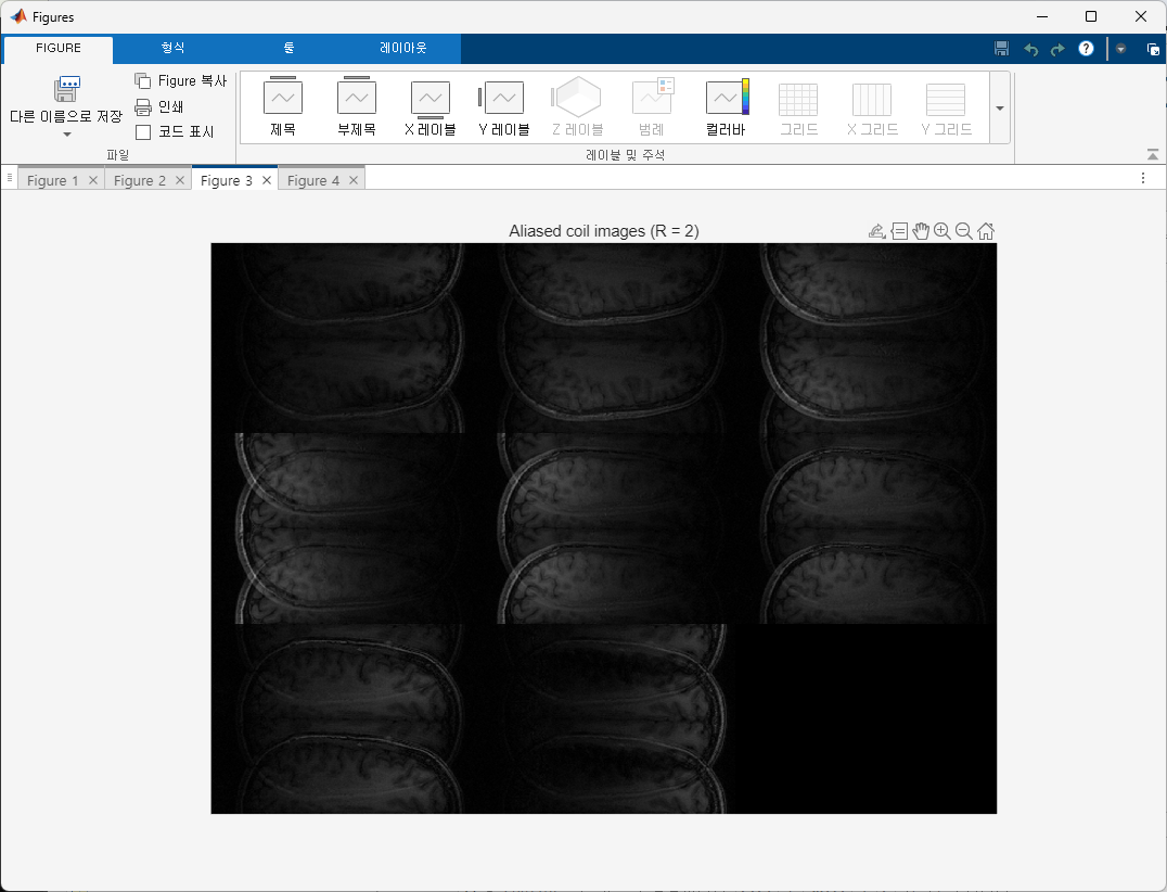
figure;
montage(permute(abs(im_us), [1, 2, 4, 3]));
title('Aliased coil images (R = 2)');

%% 3. SENSE 복원  (슬라이드 식: sol = (A^T A)^(-1) A^T b)
sep = Nx / R;                       % 겹치는 두 픽셀의 간격 (행 방향)

im_sense = zeros(Nx, Ny);           % 복원된 단일 이미지 (complex)

for iy = 1:Ny                    % 열 고정
    for ix_us = 1:Nx             % alias 가 걸린 행 인덱스

        % 이 alias 픽셀에 겹쳐진 실제 위치 인덱스들 (행 방향 wrap-around)
        orig_idx = ix_us + (0:R-1) * sep;      % [ix, ix+sep]
        orig_idx(orig_idx > Nx) = orig_idx(orig_idx > Nx) - Nx;

        % b : 각 coil에서 측정된 alias 값 F_i  (Nc x 1)
        b = squeeze(im_us(ix_us, iy, :));      % [Nc, 1]

        % A : coil sensitivity matrix  (Nc x R)
        A = zeros(Nc, R);
        for r = 1:R
            A(:, r) = squeeze(map(orig_idx(r), iy, :));   % [Nc, 1]
        end

        % 슬라이드 식: sol = (A^T A)^(-1) A^T b
        sol = pinv(A' * A) * (A' * b);         % [R, 1] = [I_A; I_B]

        % 복원 값 채워 넣기
        im_sense(orig_idx, iy) = sol;
    end
end


%% 4. 결과 표시
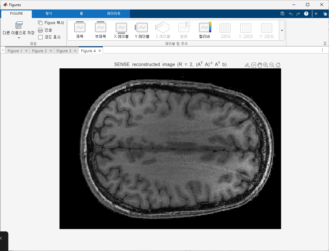
figure;
imshow(permute(abs(im_sense), [1, 2, 4, 3]), []);
title('SENSE reconstructed image (R = 2, (A^T A)^{-1} A^T b)');

%
% % Q1
% clear all; close all; clc;
%
% % (128, 128)
% % Image_NZP(ver. Non-Zero-Padding)
% I_NZP = double(phantom(128));
% I_NZP = I_NZP/max(I_NZP(:));
% Size_I_NZP = max(size(I_NZP, 1), size(I_NZP, 2));
%
% % Image_NZP Index 좌표(ver. Non-Zero-Padding)
% [Ny_NZP, Nx_NZP] = size(I_NZP);
% cx_NZP = floor(Nx_NZP/2) + 1; % Image_NZP 중앙 x 인덱스
% cy_NZP = floor(Ny_NZP/2) + 1; % Image_NZP 중앙 y 인덱스
%
% % Image_ZP Index 좌표(ver. Zero-Padding)
% I_ZP = zeros([256, 256]); % 가로 256줄 세로 256줄
% [Ny_ZP, Nx_ZP] = size(I_ZP);
% cx_ZP = floor(Nx_ZP/2) + 1; % Image_ZP 중앙 x 인덱스
% cy_ZP = floor(Ny_ZP/2) + 1; % Image_ZP 중앙 y 인덱스
%
% % Image_ZP(ver. Zero-Padding)
% I_ZP(cy_ZP-Ny_NZP/2+1:cy_ZP+Ny_NZP/2, ...
%      cx_ZP-Nx_NZP/2+1:cx_ZP+Nx_NZP/2) = I_NZP;
% Size_I_ZP = max(size(I_ZP, 1), size(I_ZP, 2));
%
% % 각도 조정
% Del_Theta = 1;
% Theta = 0:Del_Theta:180-Del_Theta;
% num_angles = length(Theta);
%
% % Sinogram 생성 (Non-Zero-Padding)
% proj1 = zeros(Size_I_NZP, num_angles);
% for i = 1:num_angles
%     proj1(:,i) = sum(imrotate(I_NZP, -Theta(i), ...
%                      'bilinear', 'crop'), 1);
% end
%
% % Sinogram 생성 (Zero-Padding) - 여기서는 참고용
% proj2 = zeros(Size_I_ZP, num_angles);
% for i = 1:num_angles
%     proj2(:,i) = sum(imrotate(I_ZP, -Theta(i), ...
%                      'bilinear', 'crop'), 1);
% end

% %%%%%%%%%%%%%%% Sinogram 시각화 %%%%%%%%%%%%%%%
%
% figure;
% subplot(1, 2, 1)
% imagesc(Theta, 1:Size_I_NZP, proj1);
% colormap gray; colorbar;
% xlabel('\theta (deg)');
% ylabel('Detector index');
% title('Sinogram (Non-Zero-Padding)');
%
% subplot(1, 2, 2)
% imagesc(Theta, 1:Size_I_ZP, proj2);
% colormap gray; colorbar;
% xlabel('\theta (deg)');
% ylabel('Detector index');
% title('Sinogram (Zero-Padding)');


% %%%%%%%%%%%%%%%%%%%%%%%%%%%%%%%%%%%%%%%%%%%%%%%%%%%%%%%%%%%%%%
% %% [중심 절편 정리(Central Slice Theorem) 수치 검증]
% %%%%%%%%%%%%%%%%%%%%%%%%%%%%%%%%%%%%%%%%%%%%%%%%%%%%%%%%%%%%%%
%
% % 1) 원본 영상의 2D Fourier Transform 계산
% F2 = fftshift(fft2(I_NZP));  % 2D FFT (center-shifted)
%
% N = Size_I_NZP;              % 128
% % 주파수 좌표계 (정수 인덱스 기반, -N/2 ~ N/2-1)
% freq = (-N/2):(N/2-1);
% [FX, FY] = meshgrid(freq, freq);  % FX: x축 방향 주파수, FY: y축 방향 주파수
%
% % 2) 비교하고 싶은 각도 (deg)
% theta_target = 30;   % 예: 30도
% [~, idx_theta] = min(abs(Theta - theta_target));
%
% % 해당 각도의 projection (spatial domain)
% p = proj1(:, idx_theta);   % N x 1
%
% % 3) projection에 대한 1D Fourier Transform (r 방향)
% P1 = fftshift(fft(p));      % N x 1, 중심 shift
%
% % 4) 2D Fourier domain에서 theta 방향 중심선 추출
% theta_rad = deg2rad(theta_target);
%
% % 중심에서 바깥으로 나가는 radius 샘플 (N개)
% rho = linspace(-N/2, N/2-1, N);   % 주파수 축과 맞추기 위한 샘플
%
% % 각 rho에 대해 (kx, ky) = (rho*cosθ, rho*sinθ)
% kx = rho * cos(theta_rad);   % 1 x N
% ky = rho * sin(theta_rad);   % 1 x N
%
% % 2D FFT에서 (kx, ky) 위치를 선형 보간 (interp2)
% % FX, FY 의 (정수 격자) 위에 F2가 있으므로, (kx, ky)는 실수 좌표 → 보간 필요
% F_line = interp2(FX, FY, F2, kx, ky, 'linear', 0);  % 1 x N
%
% % 5) 크기 정규화 후 비교
% P1_mag     = abs(P1);
% F_line_mag = abs(F_line(:));   % 열벡터로
%
% % 정규화 (최댓값 1)
% P1_mag     = P1_mag     / max(P1_mag);
% F_line_mag = F_line_mag / max(F_line_mag);
%
% % 6) 플롯으로 확인
% figure;
% subplot(2,1,1);
% plot(rho, P1_mag, 'b-o', 'DisplayName','|FFT(Projection)|');
% hold on;
% plot(rho, F_line_mag, 'r-*', 'DisplayName','|2D FFT line|');
% xlabel('Frequency index (rho)');
% ylabel('Normalized magnitude');
% title(sprintf('Central Slice Theorem Check (\\theta = %.1f^\\circ)', Theta(idx_theta)));
% legend; grid on;
%
% % 7) 차이(오차) 확인
% subplot(2,1,2);
% plot(rho, P1_mag - F_line_mag, 'k-o');
% xlabel('Frequency index (rho)');
% ylabel('Difference');
% title('Difference: |FFT(Projection)| - |F2 line|');
% grid on;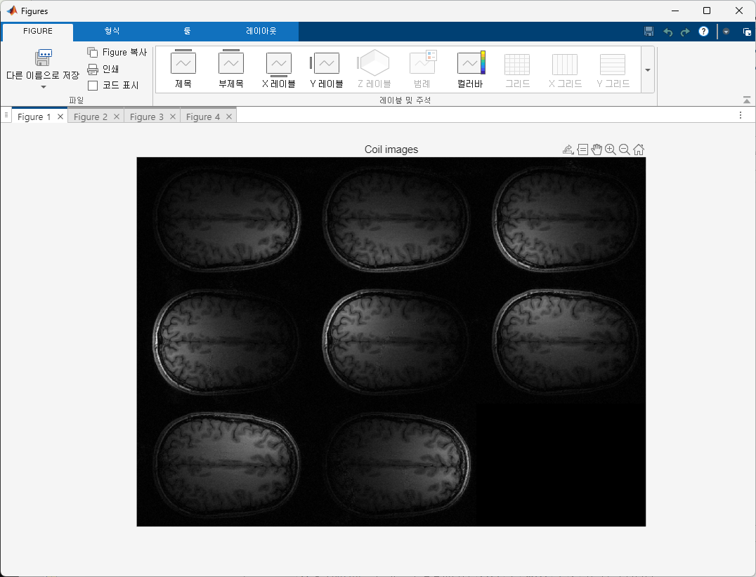
만약에 x축 방향 복원 원한다면
%% 3. SENSE 복원  (가로 방향 alias 기준)

sep = Ny / R;                       % 겹치는 두 픽셀의 간격 (열 방향)

im_sense = zeros(Nx, Ny);           % 복원된 단일 이미지 (complex)

for ix = 1:Nx                    % 행 고정
    for iy_us = 1:Ny             % alias 가 걸린 열 인덱스

        % 이 alias 픽셀에 겹쳐진 실제 위치 인덱스들 (열 방향 wrap-around)
        orig_idx = iy_us + (0:R-1) * sep;      % [iy, iy+sep]
        orig_idx(orig_idx > Ny) = orig_idx(orig_idx > Ny) - Ny;

        % b : 각 coil에서 측정된 alias 값 F_i  (Nc x 1)
        b = squeeze(im_us(ix, iy_us, :));      % [Nc, 1]

        % A : coil sensitivity matrix  (Nc x R)
        A = zeros(Nc, R);
        for r = 1:R
            A(:, r) = squeeze(map(ix, orig_idx(r), :));   % [Nc, 1]
        end

        % 슬라이드 식: sol = (A^T A)^(-1) A^T b
        sol = pinv(A' * A) * (A' * b);         % [R, 1]

        % 복원 값 채워 넣기 (열 방향으로)
        im_sense(ix, orig_idx) = sol;
    end
end
MRI 설명
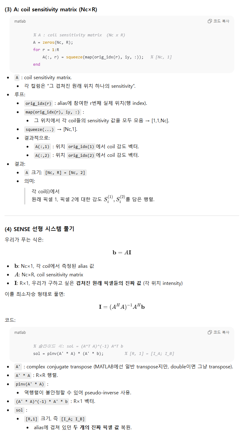
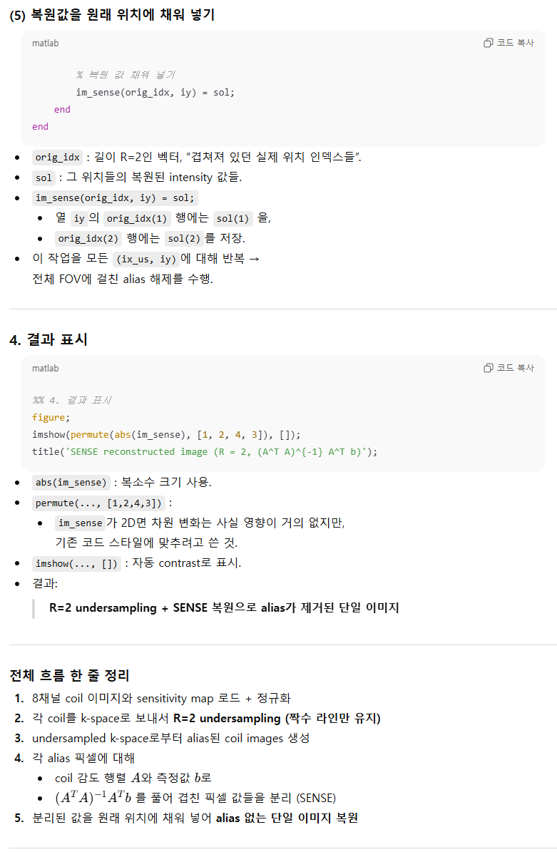
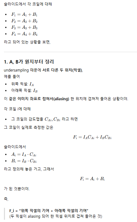
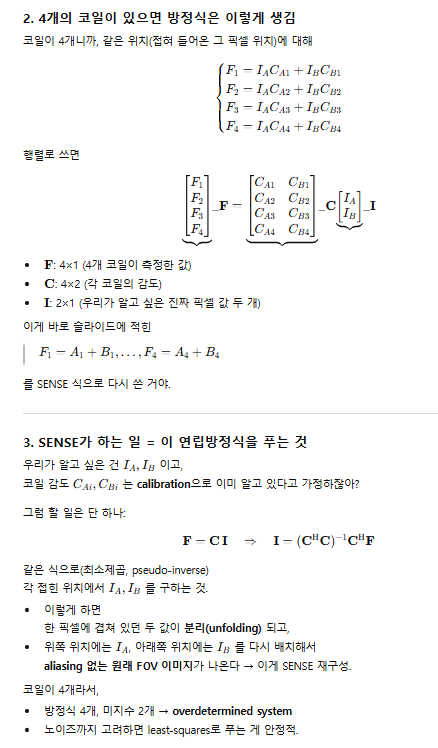
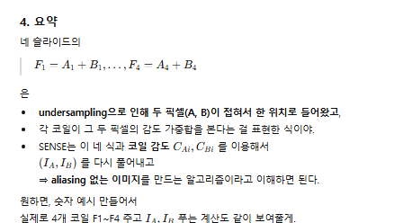
기타
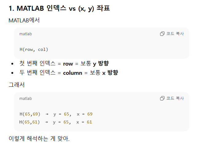
좋아, 이건 가우시안 잡음의 분포랑 파워 스펙트럼(PSD)을 확인하는 코드야.
위에서부터 차근차근 볼게.

clear; close all;
im_size = 128;
N = 1000;


clear; : 워크스페이스 변수 삭제

close all; : 열려 있는 figure 창 모두 닫기

im_size = 128; : 영상 크기 128×128로 설정

N = 1000; : 잡음(realization) 을 1000장 생성하겠다는 의미 (3차원 배열의 3번째 축)

p = phantom(im_size);


phantom(im_size) : Shepp-Logan 팬텀(CT 실습에서 많이 쓰는 그 타원형 머리 모양)을
128×128 크기로 생성

p : 깨끗한(노이즈 없는) 원본 영상

noise = 0.5*randn(im_size,im_size,N);


randn(im_size,im_size,N) :
평균 0, 분산 1인 가우시안 랜덤 값들을
128 × 128 × 1000 크기로 생성

0.5*randn(...) : 표준편차가 0.5인 가우시안 노이즈
→ 즉, noise 는 크기가 [128, 128, 1000] 인 3D 배열 (프레임 1000장)

figure, hist(noise(:),100)
xlabel('Noise Signal');
ylabel('Noise Histogram');


noise(:) : 3D 배열을 1D 벡터로 펼침 → 모든 픽셀의 노이즈 값

hist(noise(:),100) :
노이즈 값 전체에 대해 bin 100개짜리 히스토그램 그림

→ 이걸로 실제로 가우시안 분포 모양이 잘 나오는지 확인하는 것

xlabel, ylabel : x축, y축 레이블

(위 코드에서 작은 따옴표는 ' 로 써야 함. 지금은 워드에서 복붙된 것처럼 보이는 유니코드 따옴표라 MATLAB에선 에러 날 수 있음)

p_n = repmat(p,[1,1,N]) + noise;


repmat(p,[1,1,N]) :
원래 p는 128×128 한 장짜리인데, 이걸 3차원으로 N번 복제
→ 크기 [128, 128, N] 인 “같은 팬텀 영상 1000장”

+ noise : 각 프레임마다 가우시안 노이즈를 더함
→ p_n(:,:,k) = 팬텀 + 잡음 이 된 noisy phantom 영상

figure,
montage(permute(p_n(:,:,1:10),[1,2,4,3]))


p_n(:,:,1:10) : 앞에서 만든 noisy phantom 중 첫 10장만 사용

permute(...,[1,2,4,3]) :
montage는 보통 [행, 열, 채널, 프레임] 형식을 기대하는데,
현재 p_n은 [행, 열, 프레임]이라서
차원 순서를 바꿔서 montage가 이해할 수 있게 맞춰줌

montage(...) : 첫 10장의 noisy phantom을 한 화면에 나열해서 보여줌
→ “노이즈가 섞인 영상들이 어떤 모습인지” 직관적으로 확인

f_noise = fftshift(fft2(fftshift(noise)));


여기가 핵심 부분이야. 노이즈의 2D 푸리에 변환을 구하는 부분.

fftshift(noise) : 중심을 영상 가운데로 오게 축 이동
(다만 여기서는 3D라서 첫 두 축에 대해서 주로 의미 있음)

fft2(...) : 각 프레임(3번째 차원에 대해)마다
2D DFT 를 적용
→ 결과도 [128, 128, N] 크기의 복소수 배열

다시 fftshift(...) : DC 성분(저주파)이 배열 중앙에 오도록 shift

결과 f_noise :
각 노이즈 프레임에 대한 주파수 영역 표현

psd_noise = mean(abs(f_noise).^2,3);


abs(f_noise).^2 : 각 주파수 성분의 에너지(= |F(u,v)|²)

mean(...,3) : 3번째 차원(N 프레임)에 대해 평균
→ 프레임 1000개에 대한 평균 파워 스펙트럼 (Power Spectral Density 추정)

즉,

같은 통계 특성을 가진 잡음을 여러 번 발생시키고,
그 푸리에 변환의 제곱 크기를 평균내서 PSD를 추정

figure,
plot((-im_size/2:im_size/2-1)/im_size, 10*log10(psd_noise(im_size/2+1,:)));
xlabel('Normalized Spatial Frequency')
ylabel('Noise PSD (dB)');
ylim([0 50])


여기서 줄 바꿈이 약간 깨진 것 같은데, 정석 형태는 보통 이렇게 쓸 거야:

plot((-im_size/2:im_size/2-1)/im_size, 10*log10(psd_noise(im_size/2+1,:)));


설명하면:

(-im_size/2:im_size/2-1)/im_size :
x축 → 정규화된 공간 주파수(normalized spatial frequency)
-128/2 ~ 128/2-1 ⇒ -64 ~ 63
이를 128로 나눠서 -0.5 ~ 0.492... 범위가 됨

psd_noise(im_size/2+1,:) :
psd_noise의 중심 행(64+1=65번째 행) 을 1D로 잘라냄
→ 즉, 주파수 평면에서 가로 방향 한 줄의 PSD 를 뽑아온 것
(주파수 u축에 대한 PSD 프로파일이라고 보면 됨)

10*log10(...) : 선형 스케일 파워 → dB 스케일로 변환

ylim([0 50]) : y축 범위를 0~50 dB로 고정
→ 플랫한(white noise에 가까운) PSD가 잘 보이도록 조정

이 코드 전체의 목적 요약

가우시안 잡음 생성

평균 0, σ = 0.5인 2D 가우시안 노이즈를 1000장 생성

노이즈 분포 확인

hist(noise(:),100) 으로 실제 샘플의 히스토그램이
가우시안 분포처럼 나오는지 확인

노이즈가 섞인 팬텀 영상 확인

montage로 noisy phantom 여러 장을 시각적으로 확인

PSD 추정 및 시각화

노이즈의 2D FFT → |F|² → 프레임 평균 → PSD 추정

가운데 행을 잘라서 normalized frequency vs PSD(dB)를 그림

화이트 노이즈라면 PSD가 주파수에 따라 거의 평탄(flat)하게 나와야 함
→ 이걸 실험적으로 보여주는 코드
function img = my_fbp(proj, Theta, filter_type, out_size)
my_fbp : 필터드 백프로젝션을 수행하는 사용자 정의 함수.
입력:
proj : sinogram (크기: N × num_angles). 각 열이 한 각도에서의 projection.
Theta : 각 projection에 대응하는 각도(벡터, 길이 = num_angles, 보통 도 단위).
filter_type : 필터 종류 ('none', 'ram-lak', 'hann' 등).
out_size : 최종 출력 이미지 크기 (out_size × out_size).
출력:
img : 복원된 CT 이미지.
matlab
코드 복사
[N, num_angles] = size(proj);
proj 의 크기를 가져옴.
N : 검출기(detector) 개수 (또는 projection의 샘플 수, 세로 크기).
num_angles : 투영 각도 개수 (열 개수).
matlab
코드 복사
% 주파수 필터 만들기
n = (-N/2 : N/2-1)';
freq = n / (N/2);
주파수 축 인덱스를 만드는 부분.
(-N/2 : N/2-1) : 길이 N인 대칭 인덱스 벡터 (예: N=128 → -64~63).
' : 열 벡터로 만들기 (N×1).
freq = n / (N/2);
freq 는 정규화된 주파수 (대략 -1 ~ 1 사이).
이후 Ram-Lak, Hann 등 필터를 freq에 대해 정의하기 위해 사용.
matlab
코드 복사
switch lower(filter_type)
case 'none'
H = ones(N,1);
case 'ram-lak'
H = abs(freq); % Ram-Lak
case 'hann'
H = abs(freq) .* (0.5 + 0.5*cos(pi*freq)); % Hann windowed Ram-Lak
otherwise
error('Unknown filter type: %s', filter_type);
end
filter_type 문자열을 소문자로 바꿔 (lower) 어떤 필터를 쓸지 선택.
case 'none'
H = ones(N,1);
필터를 모두 1로 → 필터링 안 함 (그냥 백프로젝션 → 단순 Back Projection).
case 'ram-lak'
H = abs(freq);
Ram-Lak 필터 (|ω|에 비례하는 고역 통과 성격의 필터).
FBP에서 가장 기본적으로 쓰이는 필터.
case 'hann'
H = abs(freq) .* (0.5 + 0.5*cos(pi*freq));
Ram-Lak(=abs(freq))에 Hann 윈도우 (0.5 + 0.5*cos(pi*freq))를 곱한 것.
고주파 쪽을 부드럽게 줄여서 노이즈를 완화하는 역할.
otherwise
정의되지 않은 필터 이름이 들어오면 에러 발생.
matlab
코드 복사
% sinogram을 주파수 영역에서 필터링
% FFT (detector 방향: 행 방향)
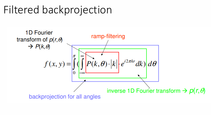
P = fftshift(fft(fftshift(proj,1), [], 1), 1);
sinogram을 주파수 영역으로 변환하는 부분.
fftshift(proj,1)
행 방향(검출기 방향, N축)에 대해 중심을 0 주파수 기준으로 shift.
fft(..., [], 1)
각 열(각각의 투영)에 대해 행 방향으로 1D FFT 수행.
다시 fftshift(...,1)
FFT 결과를 또 한 번 shift 해서 DC(0주파수)가 가운데 오도록 정렬.
결과 P :
크기 N × num_angles
각 열은 한 projection의 주파수 스펙트럼.
matlab
코드 복사
% 필터 적용
P_filtered = P .* H;
H : N×1 필터.
P : N×num_angles.
브로드캐스팅(또는 implicit expansion)으로 각 열마다 같은 필터 H를 곱함.
즉, 각 투영의 주파수 성분에 필터를 곱해줌.
matlab
코드 복사
% IFFT
proj_filtered = real(ifftshift(ifft(ifftshift(P_filtered,1), [], 1),1));
필터링된 주파수 데이터를 다시 공간 영역으로 되돌리는 단계.
ifftshift(P_filtered,1)
FFT에서 shift 했던 걸 되돌린 후,
ifft(..., [], 1)
행 방향으로 1D inverse FFT.
ifftshift(...,1)
다시 중앙 기준으로 shift (표현 정렬용).
real(...)
수치 오차 때문에 생긴 미세한 허수 성분 제거 → 실제(real) 값만 사용.
결과 proj_filtered :
필터링된 sinogram (공간 도메인), 크기 N × num_angles.
matlab
코드 복사
% Backprojection
img_bp = zeros(N, N);
백프로젝션으로 누적할 이미지를 0으로 초기화.
크기 N × N인 reconstruction 공간.
matlab
코드 복사
for i = 1:num_angles
col = proj_filtered(:, i);
row = col';
bp_slice = repmat(row, N, 1);
bp_rot = imrotate(bp_slice, Theta(i), 'bilinear', 'crop');
img_bp = img_bp + bp_rot;
end
각 줄 설명:
for i = 1:num_angles
각 각도 Theta(i) 에 대해 한 번씩 백프로젝션.
col = proj_filtered(:, i);
i번째 각도에서의 필터링된 projection 한 줄(N×1) 가져오기.
row = col';
행 벡터(1×N)로 전치.
bp_slice = repmat(row, N, 1);
row를 N번 반복해서 N×N 이미지로 확장.
즉, “같은 projection 값을 각 행에 그대로 복사해서 채운 2D 슬라이스”
→ 특정 각도에서의 projection을 x축 방향으로 펼쳐 놓은 형태.
bp_rot = imrotate(bp_slice, Theta(i), 'bilinear', 'crop');
이 bp_slice를 Theta(i)만큼 회전시킴.
'bilinear' : 회전할 때 bilinear interpolation 사용.
'crop' : 회전 후, 결과를 원래 크기(N×N)에 맞게 잘라냄.
의미상으로는:
i번째 projection을 해당 각도로 역투영(backproject)한 2D 이미지.
img_bp = img_bp + bp_rot;
현재 각도에서의 backprojection 결과를 전체 이미지에 누적.
모든 각도에 대해 이런 식으로 합쳐서 최종 복원.
matlab
코드 복사
img_bp = img_bp * (pi / (2 * num_angles));
백프로젝션 후 스케일 정규화.
FBP 이론에서, 연속적인 θ에 대한 적분(0~π)을
유한한 num_angles 개의 각도에 대한 합으로 근사할 때 붙는 계수.
대략적으로
img
≈
𝜋
2
⋅
num_angles
∑
𝑖
backprojection at
Θ
𝑖
img≈
2⋅num_angles
π
i
∑
backprojection at Θ
i
이런 식의 보정.
matlab
코드 복사
if N ~= out_size
start = floor((N - out_size)/2) + 1;
img = img_bp(start:start+out_size-1, start:start+out_size-1);
else
img = img_bp;
end
end
최종적으로 중앙 부분만 잘라서 원하는 크기로 맞추는 부분.
if N ~= out_size
복원된 이미지 크기 N×N이 원하는 출력 사이즈와 다를 경우.
start = floor((N - out_size)/2) + 1;
중앙에서 out_size 크기로 잘라내기 위한 시작 인덱스 계산.
예: N=128, out_size=100 이면 → (128-100)/2 = 14 → start = 15.
img = img_bp(start:start+out_size-1, start:start+out_size-1);
중앙 기준으로 out_size × out_size 영역만 crop.
else
이미 N == out_size라면 그대로 반환.
end
함수 끝.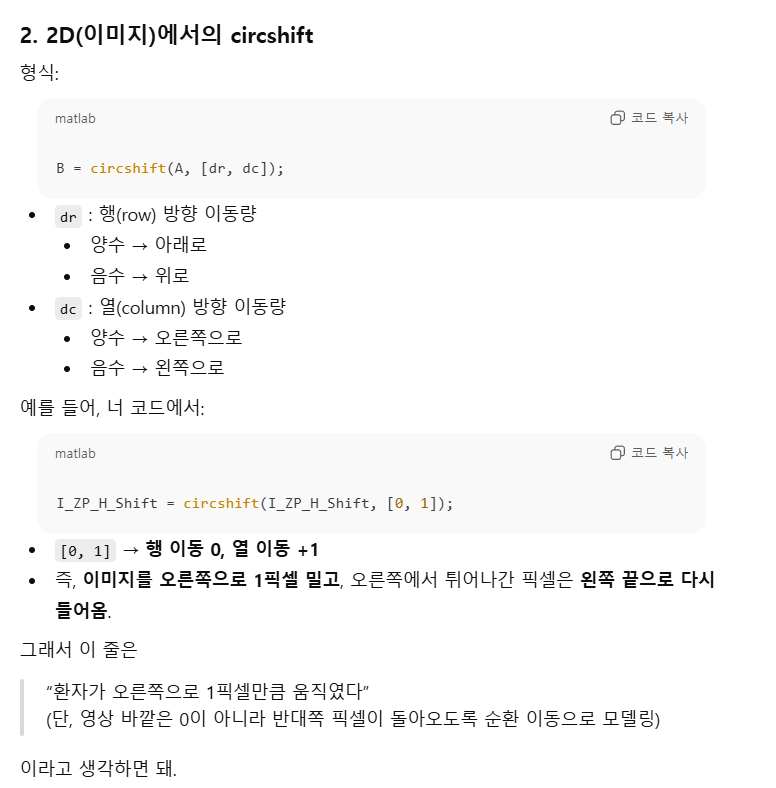
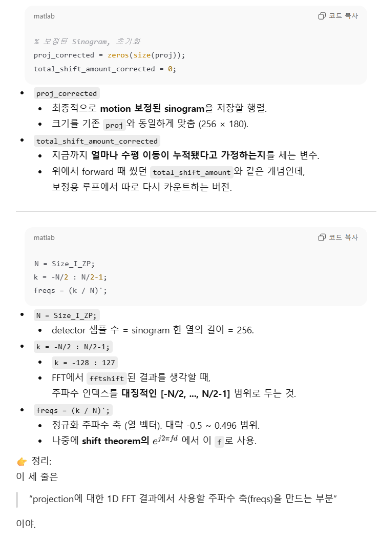
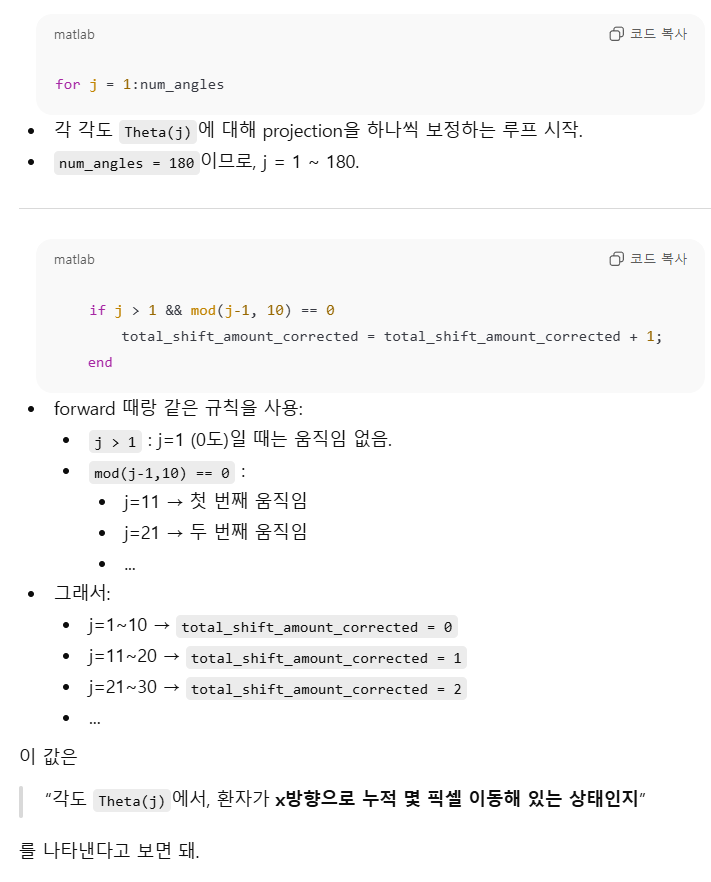
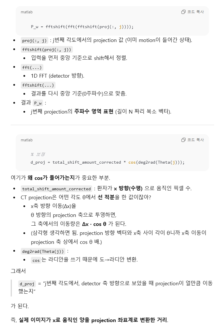
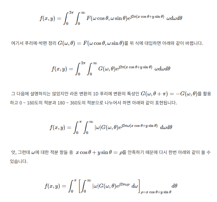
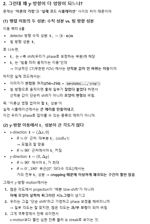
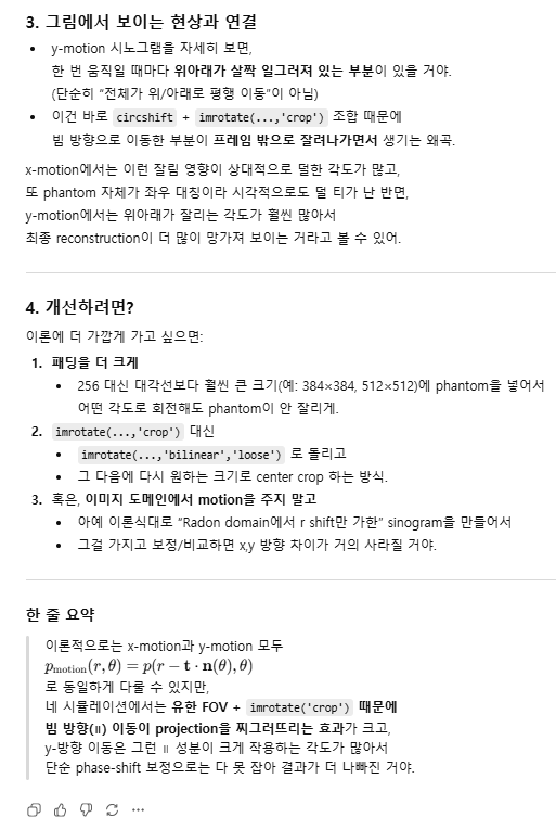
cos 함수 곱하는거 보충 설명!!!!!
(만약에 y축으로 움직이면 cos 대신 sin을 넣으면 되겠구나!!)
근데 잘 안된다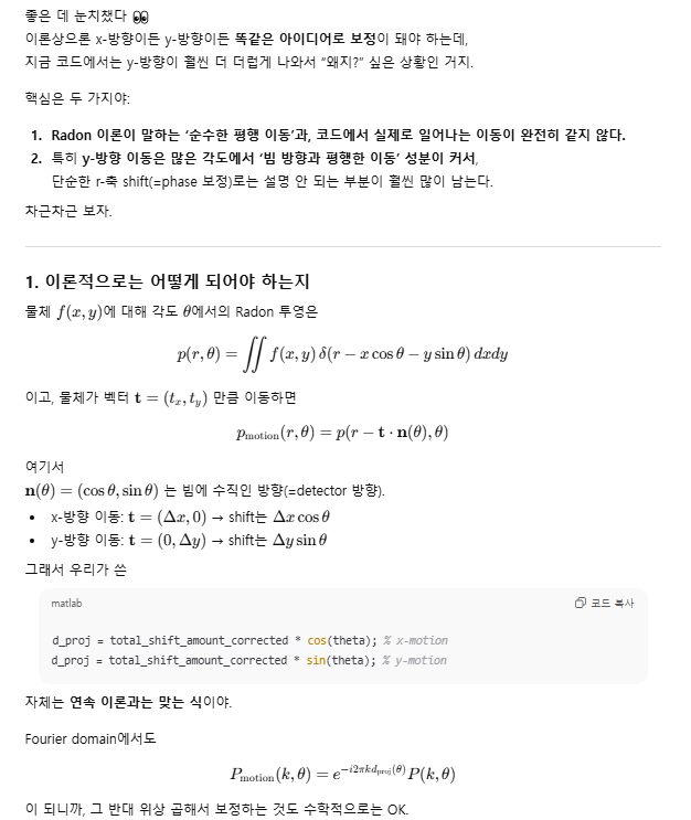
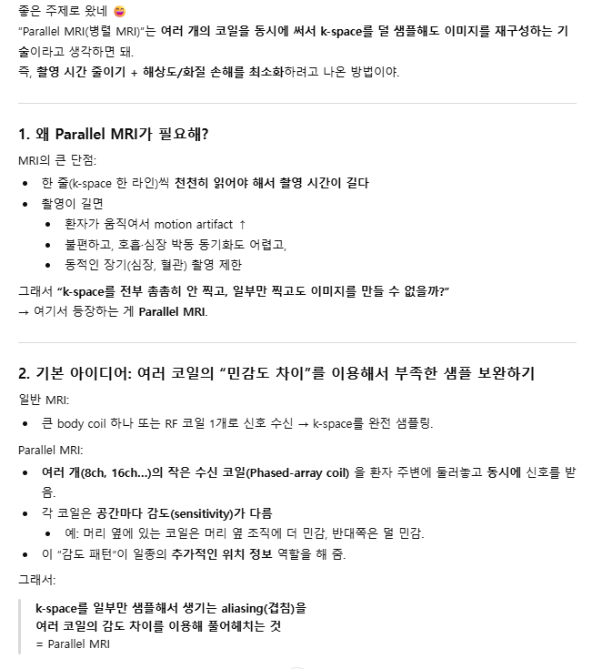
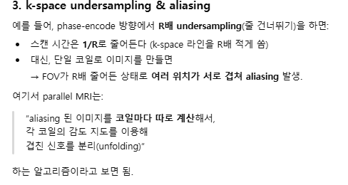
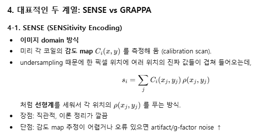
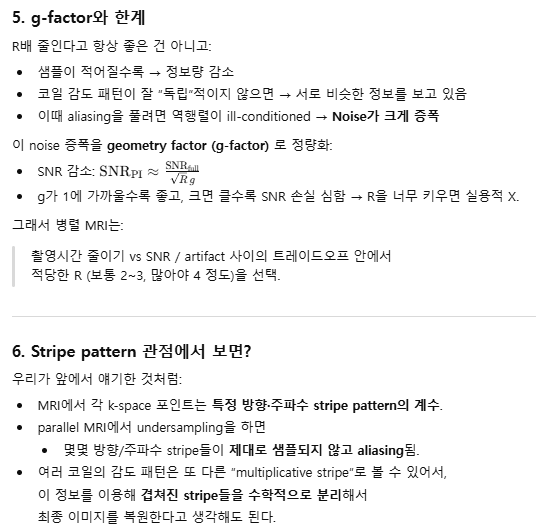
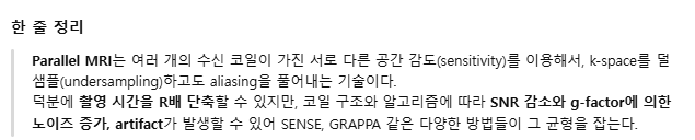
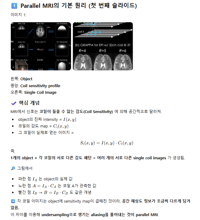
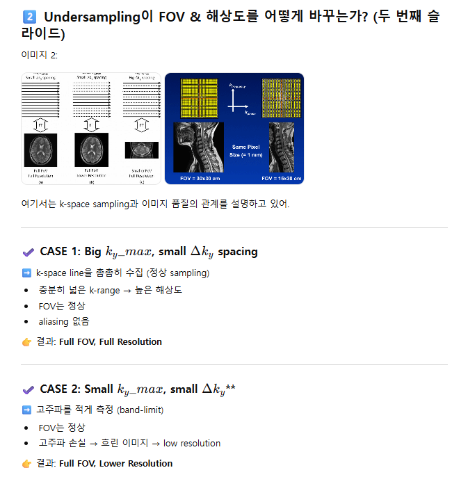
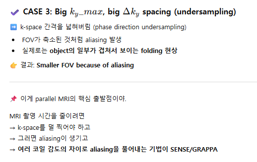
Parallel MRI
한 단면 투영
%%%%%%%%%%%%%%%%%%%%%

% 보고 싶은 각도
theta_target = 90;  % [deg]

% 해당 각도의 인덱스 찾기
[~, idx_theta] = min(abs(Theta - theta_target));

% Non-Zero-Padding sinogram에서 한 단면(컬럼) 보기
figure;
plot(1:Size_I_NZP, proj1(:, idx_theta), '-o');
xlabel('Detector index');
ylabel('Projection value');
title(sprintf('Projection at \\theta = %.1f^\\circ (Non-Zero-Padding)', Theta(idx_theta)));
grid on;


% 가운데 Detector index
det_idx = round(Size_I_NZP/2);

% Non-Zero-Padding sinogram에서 한 행(row) 보기
figure;
plot(Theta, proj1(det_idx, :), '-o');
xlabel('\theta (deg)');
ylabel('Projection value');
title(sprintf('Sinogram row at detector index = %d (Non-Zero-Padding)', det_idx));
grid on;

p_single = proj1(:, idx_theta);                 % M x 1
sino_single = p_single;                         % M x 1 그대로
theta_single = Theta(idx_theta);                % 1 x 1

I_bp_iradon = iradon(sino_single, theta_single, ...
                     'linear', 'none', 1, Size_I_NZP);

figure; imagesc(I_bp_iradon); axis image off; colormap gray;
title('iradon으로 한 각도만 역투영');
colorbar;


% --------------------------
% 1) 사용할 각도 선택
% --------------------------
theta_target = 90;  % 원하는 각도 (deg)
[~, idx_theta] = min(abs(Theta - theta_target));  % 가장 가까운 각도의 인덱스

% 해당 각도의 프로젝션 (1D 벡터)
p = proj1(:, idx_theta);   % Size_I_NZP x 1

% --------------------------
% 2) 1D 프로젝션을 2D 스트립으로 확장
%    -> 각 컬럼마다 p(j) 값이 세로로 쭉 복사된 이미지
% --------------------------
strip = repmat(p', Size_I_NZP, 1);   % (행: y 방향, 열: detector index)

% --------------------------
% 3) 스트립을 다시 +theta 만큼 회전 (역투영)
% --------------------------
bp_single = imrotate(strip, Theta(idx_theta), 'bilinear', 'crop');

% --------------------------
% 4) 결과 보기
% --------------------------
figure;
subplot(1,3,1);
imagesc(I_NZP); axis image off; colormap gray;
title('원본 팬텀');

subplot(1,3,2);
plot(p); xlim([1 Size_I_NZP]);
title(sprintf('Projection at \\theta = %.1f^\\circ', Theta(idx_theta)));
xlabel('Detector index'); ylabel('Value'); grid on;

subplot(1,3,3);
imagesc(bp_single); axis image off; colormap gray;
title(sprintf('Backprojection (Single Angle: %.1f^\\circ)', Theta(idx_theta)));
colorbar;