DIP : Mid-Term Exam

LMS에서 과제 및 강의 자료 미리 다운로드 해놓기
틀린 Code 있을 수 있으니까, 형태만 사용하고, 참고만 하기!!
https://everyday-image-processing.tistory.com/category/image%20processing
https://monee1001.tistory.com/15
https://infograph.tistory.com/271
HW1
Q1.5(a)
freq = 0.005
n = 0:1:199
k = 1:1:10
x_n = cos(2*pi*freq*n)

plot(n, x_n)

xlabel('n')
ylabel('x(n)')
title('Cosine Function')
grid on
Q1.5(b)
freq = 0.005
% n = 0:1:199
n = -199:1:199
k = 1:1:10
sum_x_n = sum(cos(2*pi*freq*(k'*n)))
scaled_sum_x_n = sum_x_n/10

% plot(n, sum_x_n)
plot(n, scaled_sum_x_n)

xlabel('n')
ylabel('x(n)')
title('Form of a Sinc Function')
grid on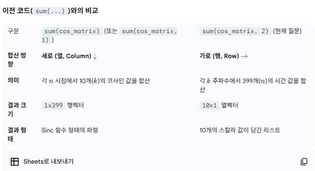
HW2
Q2.1
A = [3, 7, -4, 12 ; -5, 9, 10, 2 ; 6, 13, 8, 11 ; 15, 5, 4, 1]

V = A(:, 2)
% V = A(2, :)
a = A(end, end)
Q2.2
A = [1, 4, 2 ; 2, 4, 100 ; 7, 9, 7 ; 3, pi, 42]
B = log(A)

% V = sum(B(2,:))
% V = B(:,2).*A(:,1)
% V = A(:,1).*B(:,2)

% V = A*B
V1 = A.*B
V2 = A'*B
V3 = A*B'
Q2.3
x_a = -2*pi : pi :2*pi
f_x_a = 3*x_a.*(cos(x_a)).^2-2*x_a

x_b = -2*pi : 0.1*pi :2*pi
f_x_b = 3*x_b.*(cos(x_b)).^2-2*x_b

x_c = -2*pi : 0.01*pi :2*pi
f_x_c = 3*x_c.*(cos(x_c)).^2-2*x_c

subplot(1, 3, 1)
plot(x_a, f_x_a)
grid on;
xlabel('x');
ylabel('f(x)');
title('Plot of f(x) = 3x(cos(x))^2 - 2x | the increment of x by pi');

subplot(1, 3, 2)
plot(x_b, f_x_b)
grid on;
xlabel('x');
ylabel('f(x)');
title('Plot of f(x) = 3x(cos(x))^2 - 2x | the increment of x by 0.1pi');

subplot(1, 3, 3)
plot(x_c, f_x_c)
grid on;
xlabel('x');
ylabel('f(x)');
title('Plot of f(x) = 3x(cos(x))^2 - 2x | the increment of x by 0.01pi');
Q2.4
x = -5 - 8j
y = 10 - 5j

xy = x*y
abs_a = abs(xy)
ang_a = angle(xy)

% abs_b = sqrt(real(xy).^2 + imag(xy).^2)
% ang_b = atan2(imag(xy), real(xy))
% ang_b_1 = atan(imag(xy)/real(xy)) % 4분면 정보를 잃음 : 그래서 의도한 값 X
Q2.5
x = linspace(0, 5)
f = @(x) 1 - 3.*x.*exp(-x)   % 함수 핸들

plot(x, f(x))
xlabel('x');
ylabel('f(x)');
title('Plot of y = 1 - 3*x*exp(-x)');
grid on;

[x_min, y_min] = fminsearch(f, 3)
disp([x_min, y_min])

% fzero(f, 0.5)
% fzero(f, 1.5)
Q2.6
t = 0:0.01:1
f = [1, 2, 5]

% my_cos = @(t,f) cos(2*pi*t.*f);

y1 = my_cos(t, f(1))
y2 = my_cos(t, f(2))
y3 = my_cos(t, f(3))

figure;
plot(t, y1); hold on;
plot(t, y2); hold on;
plot(t, y3); hold on;
grid on;
legend('1 Hz','2 Hz','5 Hz');

title('Cosine Wave for f = 1, 2, 5 Hz');
xlabel('Time(sec)');
ylabel('Amplitude');

% subplot(1, 3, 1)
% plot(t, y1);
% title('Cosine Wave for f = 1 Hz');
% xlabel('Time(sec)');
% ylabel('Amplitude');
%
% subplot(1, 3, 2)
% plot(t, y2);
% title('Cosine Wave for f = 2 Hz');
% xlabel('Time(sec)');
% ylabel('Amplitude');
%
% subplot(1, 3, 3)
% plot(t, y3);
% title('Cosine Wave for f = 5 Hz');
% xlabel('Time(sec)');
% ylabel('Amplitude');
Q2.7
t = 0 : 0.001 : 1
% t = -1 : 0.001 : 1
f = 1
n = [2, 5, 10, 20]

y1 = my_cos_sum(t, f, n(1))
y2 = my_cos_sum(t, f, n(2))
y3 = my_cos_sum(t, f, n(3))
y4 = my_cos_sum(t, f, n(4))

subplot(2, 2, 1)
plot(t, y1);
title('Cosine Wave for n = 2');
xlabel('Time (s)');
ylabel('Amplitude');

subplot(2, 2, 2)
plot(t, y2);
title('Cosine Wave for n = 5');
xlabel('Time (s)');
ylabel('Amplitude');

subplot(2, 2, 3)
plot(t, y3);
title('Cosine Wave for n = 10');
xlabel('Time (s)');
ylabel('Amplitude');

subplot(2, 2, 4)
plot(t, y4);
title('Cosine Wave for f = 20');
xlabel('Time (s)');
ylabel('Amplitude');
my_cos.m
function y = my_cos(t, f)
y = cos(2*pi*f.*t)
my_cos_sum.m
function y = my_cos_sum(t, f, n)
k = 1:1:n
y = (1/n) * sum( my_cos(t, f.*k'))
HW3
Q3.1
clear
clc

x = [10, -2, 6, 5, -3];
y = [9, -3, 2, 5, -1];

% z_a = (x < 6)
% z_b = (x <= y)
% z_c = (x == y)
z_d = (x ~= y)
Q3.2
clear
clc

x = [-3, 0, 0, 2, 5, 8];
y = [-5, -2, 0, 3, 4, 10];

% z_a = (y < ~x)
z_b = (x & y)
% z_c = (x | y)
% z_d = xor(x,y)
Q3.3
clear
clc

years= 1800:100:2500;
y = zeros(size(years));

for i = 1:numel(years)
    y(i) = check_leap_year(years(i));
end

T = table(years(:), y(:), 'VariableNames', {'Year','IsLeap'});
disp(T)
Q3.4
clear
clc

t = 0:0.1:4;
x_t = 5*t-10;
y_t = 25*t.^2-120*t+144;

% (a)
% best_distance = inf;
% best_i = 1;
% for i = 1:numel(t)
%     distance = sqrt(x_t(i).^2 + y_t(i).^2);
%     if distance <= best_distance
%         best_distance = distance;
%         best_i = i;
%     end
% end

% (b)
distance = sqrt(x_t.^2 + y_t.^2);
[best_distance, best_i] = min(distance);

t_min = t(best_i);
distance_min = best_distance;
fprintf('t = %.1f 일때, distance = %.6f 로 최솟값을 가짐\n\n', t_min, distance_min);

distance = sqrt(x_t.^2 + y_t.^2);
T = table(t(:), x_t(:), y_t(:), distance(:), 'VariableNames', {'time','x', 'y', 'distance'});
disp(T)
Q3.5
clear
clc

goal_deposit = 1000000;

initial_deposit = 10000;
annual_deposit = 10000;
interest = 0.03;

present_deposit = initial_deposit;
count_year = 0;

fprintf("초기 누적액 : %.0f 원\n", present_deposit);

while present_deposit < goal_deposit
    present_deposit = present_deposit + annual_deposit;
    present_deposit = present_deposit * (1 + interest);
    count_year = count_year + 1;
    fprintf("%d 년 뒤, 연초 누적액 : %.0f 원\n", count_year, present_deposit);
end

fprintf("소요 기간: %d 년, 최종 누적액: %.2f 원\n", count_year, present_deposit);
Q3.6
clear
clc

annual_deposits = [10000, 15000, 20000, 30000, 40000, 50000, 60000];
years = zeros(size(annual_deposits));
for i = 1:numel(years)
    years(i) = save_million(annual_deposits(i));
end
% years = arrayfun(@save_million, annual_deposits);
T = table(annual_deposits(:), years(:), 'VariableNames', {'annual_deposits','years'});
disp(T)
Q3.7
clear
clc
close

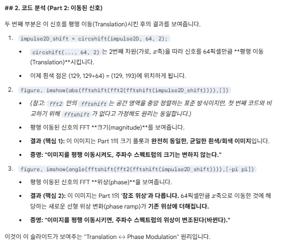
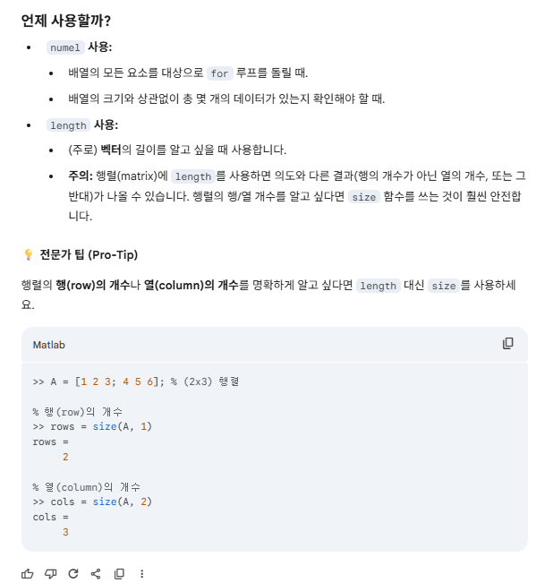
Image = phantom('Modified Shepp-Logan', 128);

F = fftshift( fft2(Image) );
% F = fft2(Image);

Mag = abs(F);
LogMag = log1p(Mag);

figure;
subplot(1,3,1)
imshow(Image,[])
title('Phantom 128×128')
colormap gray;

subplot(1,3,2)
imshow(Mag,[])
title('|F(u,v)|');

subplot(1,3,3)
imshow(LogMag,[])
title('log(1+|F|)');
save_million.m
function years = save_million(annual_deposit)
years = 0;
goal_deposit = 1000000;
present_deposit = 0;

switch true
    case annual_deposit < 10000
        compound_interest = 0;
    case annual_deposit < 20000
        compound_interest = 0.01;
    case annual_deposit < 30000
        compound_interest = 0.02;
    case annual_deposit < 40000
        compound_interest = 0.03;
    case annual_deposit < 50000
        compound_interest = 0.04;
    otherwise
        compound_interest = 0.05;
end

while present_deposit < goal_deposit
    present_deposit = present_deposit * (1 + compound_interest);
    present_deposit = present_deposit + annual_deposit;
    years = years + 1;
end
end
check_leap_year.m
function y = check_leap_year(year)
if mod(year, 4) == 0
    if mod(year, 400) == 0
        y = 1;
    elseif mod(year, 100) == 0
        y = 0;
    else
        y = 1;
    end
else
    y = 0;
end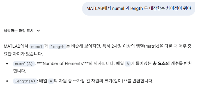
HW4
Q4.1
close all; clear; clc;

file1 = imread("Fig0208(a).tif");

fig1 = im2double(file1);
nor_fig1 = fig1 / sum(fig1(:));

figure;

subplot(3, 2, 1)
imshow(file1);
title("Original Image");

subplot(3, 2, 2)
imhist(file1);
xlim("auto"); ylim("auto"); grid on;
xlabel('Intensity'); ylabel('Counts');
title("Histogram of Original Image")

subplot(3, 2, 3)
imshow(nor_fig1);
title("Normalized Image(1)");

subplot(3, 2, 4)
hist1 = histogram(nor_fig1(:), 256, 'Normalization', 'probability');
hist1.FaceColor = 'b'; hist1.EdgeColor = 'b';
xlim("auto"); ylim([0 1]); grid on;
xlabel('Intensity'); ylabel('Probability');
title("Histogram of Normalized Image(1)");

subplot(3, 2, 5)
imshow(nor_fig1, []);
title("Normalized Image(2)");

subplot(3, 2, 6)
hist1 = histogram(nor_fig1(:), 256, 'Normalization', 'probability');
hist1.FaceColor = 'b'; hist1.EdgeColor = 'b';
xlim("auto"); ylim([0 1]); grid on;
xlabel('Intensity'); ylabel('Probability');
title("Histogram of Normalized Image(2)");
Q4.2
close all; clear; clc;

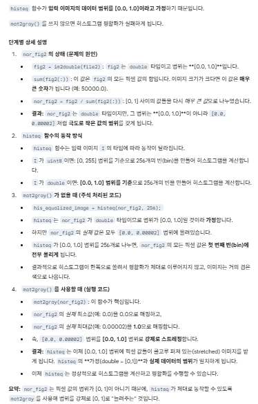
file2 = imread("Fig0208(a).tif");

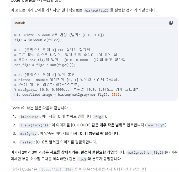
fig2 = im2double(file2);
nor_fig2 = fig2 / sum(fig2(:));

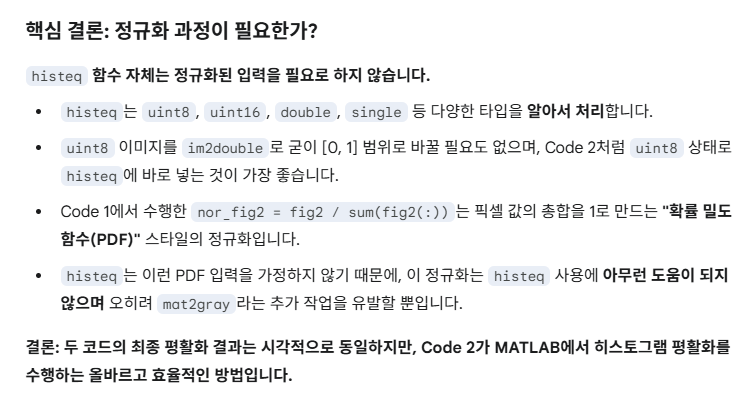
% his_equalized_image = histeq(nor_fig2, 256);
his_equalized_image = histeq(mat2gray(nor_fig2), 256);

figure;

subplot(3, 2, 1);
imshow(file2);
title("Original Image");

subplot(3, 2, 2);
imhist(file2);
xlim("auto"); ylim("auto"); grid on;
xlabel('Intensity'); ylabel('Counts');
title("Original Histogram");

subplot(3, 2, 3);
imshow(nor_fig2, []);
title("Normalized Image");

subplot(3, 2, 4)
hist1 = histogram(nor_fig2(:), 256, 'Normalization', 'probability');
hist1.FaceColor = 'b'; hist1.EdgeColor = 'b';
xlim("auto"); ylim([0 1]); grid on;
xlabel('Intensity'); ylabel('Probability');
title("Histogram of Normalized Image");

subplot(3, 2, 5);
imshow(his_equalized_image, []);
title("Histogram Equalized Image");

subplot(3, 2, 6);
hist2 = histogram(his_equalized_image(:), 256, 'Normalization', 'probability');
hist2.FaceColor = 'b'; hist2.EdgeColor = 'b';
xlim("auto"); ylim("auto"); grid on;
xlabel('Intensity'); ylabel('Probability');
title("Histogram of Histogram Equalized Image");
Q4.2-1
close all; clear; clc;

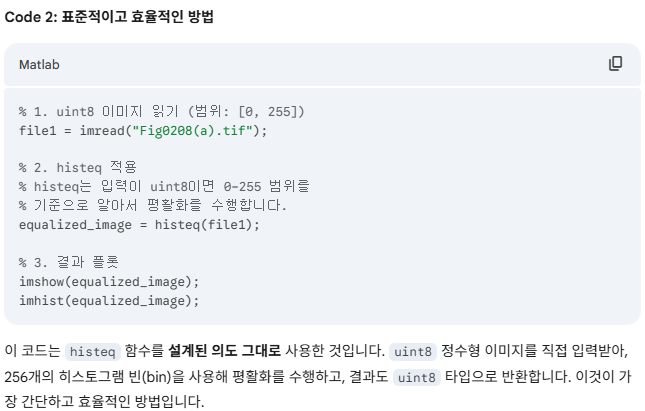
file1 = imread("Fig0208(a).tif");

equalized_image = histeq(file1);

figure;

subplot(2, 2, 1);
imshow(file1);
title("Original Image");

subplot(2, 2, 2);
imhist(file1);
title("Original Histogram");

subplot(2, 2, 3);
imshow(equalized_image);
title("Equalized Image");

subplot(2, 2, 4);
imhist(equalized_image);
title("Equalized Histogram");
Q4.3
% close all; clear; clc;
%
% file3 = imread("Fig0208(a).tif");
%
% fig3 = im2double(file3);
% nor_fig3 = fig3 / sum(fig3(:));
%
% his_equalized_image = histeq(mat2gray(nor_fig3), 256);
%
% [cnt, bins] = imhist(mat2gray(nor_fig3), 256);
% prob = cnt / sum(cnt);
% T = cumsum(prob);
%
% Ieq_manual = interp1(bins, T, mat2gray(nor_fig3), 'linear', 'extrap');
% fprintf('mean |manual - histeq| = %.3e\n', mean(abs(Ieq_manual(:)-his_equalized_image(:))));
%
% figure;
%
% subplot(1, 3, 1);
% imshow(file3);
% title("Original Image");
%
% subplot(1, 3, 2);
% imshow(nor_fig3, []);
% title("Normalized Image");
%
% subplot(1, 3, 3);
% imshow(his_equalized_image, []);
% title("Histogram Equalized Image");
%
% figure;
% plot(bins, T, 'LineWidth', 2); hold on
% plot([0 1], [0 1], '--');
% xlim("auto"); ylim("auto"); grid on;
% xlabel('Input intensity r'); ylabel('Output intensity s = T(r)');
% legend('T(r) = CDF(r)', 'y = x', 'Location','SouthEast');
% title('Intensity Transformation for Histogram Equalization:  s = T(r) = CDF(r)');

close all; clear; clc;

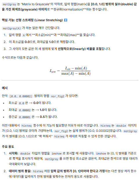
% 1. 원본 이미지를 읽고 [0, 1] 범위의 double 타입으로 변환합니다.
file3 = imread("Fig0208(a).tif");
fig3 = im2double(file3);

% 2. [0, 1] 이미지(fig3)에 바로 histeq를 적용합니다.
% 이것이 MATLAB의 표준적인 방법입니다.
his_equalized_image = histeq(fig3, 256);

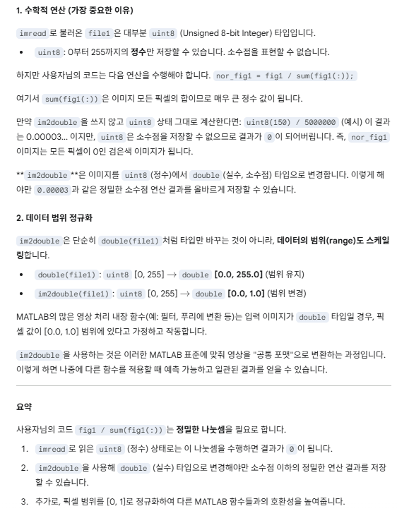
% 3. 강도 변환 함수 T(r)을 구합니다.
% T(r)은 원본 이미지(fig3)의 누적 분포 함수(CDF)입니다.
[cnt, bins] = imhist(fig3, 256); % <- 원본 fig3의 히스토그램
prob = cnt / sum(cnt);
T = cumsum(prob); % T(r) = CDF(r)

% 4. (검증) 수동으로 변환 함수 T(r)을 원본 이미지(fig3)에 적용합니다.
Ieq_manual = interp1(bins, T, fig3, 'linear', 'extrap');

% 5. (검증) 수동 변환 결과와 histeq() 내장 함수 결과를 비교합니다.
% 이 값이 0에 가까우면 T(r)을 올바르게 구했다는 의미입니다.
fprintf('mean |manual - histeq| = %.3e\n', mean(abs(Ieq_manual(:) - his_equalized_image(:))));

% 6. 이미지 결과 표시
figure;
subplot(1, 3, 1);
imshow(file3);
title("Original Image (uint8)");

subplot(1, 3, 2);
imshow(fig3, []); % [0, 1] double 이미지
title("Original Double [0, 1]");

subplot(1, 3, 3);
imshow(his_equalized_image, []);
title("Histogram Equalized Image");

% 7. 강도 변환 함수 T(r) 플롯
figure;
plot(bins, T, 'LineWidth', 2); hold on
plot([0 1], [0 1], '--');
xlim([0 1]); ylim([0 1.05]); % 축 범위를 명확하게 설정
grid on;
xlabel('Input intensity r'); ylabel('Output intensity s = T(r)');
legend('T(r) = CDF(r)', 'y = x', 'Location','SouthEast');
title('Intensity Transformation for Histogram Equalization:  s = T(r) = CDF(r)');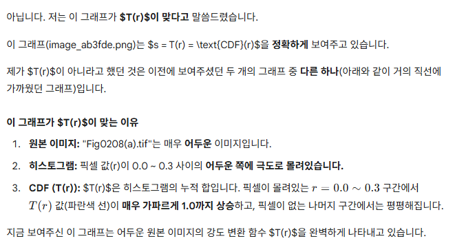
HW5
Q5.1
clear all; close all; clc

x_n_func = @(n) (n >= 0 & n <= 29);

h_n_func = @(n, N) (n >= 0 & n <= N-1);

n = 0:1:99;
N = 2;

x_n = x_n_func(n); h_n = h_n_func(n, N);

len_n = length(n); len_x = length(x_n); len_h = length(h_n);
len_y = len_x + len_h - 1;

y_n_1 = zeros(1, len_y);

for i = 1:len_x
    for j = 1:len_h
        y_n_1(i+j-1) = y_n_1(i+j-1) + x_n(i) * h_n(j);
    end
end

y_n_2 = conv(x_n, h_n);

figure;

subplot(2, 2, 1);
stem(n, x_n);
title('Input Sequence x[n]');
xlabel('n'); ylabel('x[n]'); grid on;
axis([0 len_n 0 max(x_n)*1.1]);

subplot(2, 2, 2);
stem(n, h_n);
title('Impulse Response h[n] (N = 2)');
xlabel('n'); ylabel('h[n]'); grid on;
axis([0 len_n 0 max(h_n)*1.1]);

subplot(2, 2, 3)
stem(n, y_n_1(1:len_n));
title('Output y[n] (Using For Loop)');
xlabel('n'); ylabel('y[n]'); grid on;
axis([0 len_n 0 max(y_n_1)*1.1]);

subplot(2, 2, 4)
stem(n, y_n_2(1:len_n));
title('Output y[n] (Using conv Function)');
xlabel('n'); ylabel('y[n]'); grid on;
axis([0 len_n 0 max(y_n_2)*1.1]);
Q5.2
clear all; close all; clc

x_n_func = @(n) (n >= 0 & n <= 29);

h_n_func = @(n, N) (n >= 0 & n <= N-1);

n = 0:1:99;
N = [3, 5, 10];

x_n = x_n_func(n);
h3_n = h_n_func(n, N(1));
h5_n = h_n_func(n, N(2));
h10_n = h_n_func(n, N(3));

len_n = length(n);
len_x = length(x_n);
len_h = length(h3_n); % 길이니까 무엇을 사용하던 무관.
len_y = len_x + len_h - 1;

% h_3
y_n_1_h3 = zeros(1, len_y);
for i = 1:len_x
    for j = 1:len_h
        y_n_1_h3(i+j-1) = y_n_1_h3(i+j-1) + x_n(i) * h3_n(j);
    end
end
y_n_2_h3 = conv(x_n, h3_n);

% h_5
y_n_1_h5 = zeros(1, len_y);
for i = 1:len_x
    for j = 1:len_h
        y_n_1_h5(i+j-1) = y_n_1_h5(i+j-1) + x_n(i) * h5_n(j);
    end
end
y_n_2_h5 = conv(x_n, h5_n);

% h_10
y_n_1_h10 = zeros(1, len_y);
for i = 1:len_x
    for j = 1:len_h
        y_n_1_h10(i+j-1) = y_n_1_h10(i+j-1) + x_n(i) * h10_n(j);
    end
end
y_n_2_h10 = conv(x_n, h10_n);

figure;

subplot(4, 1, 1);
stem(n, x_n);
title('Input Sequence x[n]');
xlabel('n'); ylabel('x[n]'); grid on;
axis([0 len_n 0 max(x_n)*1.1]);

subplot(4, 1, 2);
stem(n, h3_n);
title('Impulse Response h[n] (N = 3)');
xlabel('n'); ylabel('h[n]'); grid on;
axis([0 len_n 0 max(h3_n)*1.1]);

subplot(4, 1, 3);
stem(n, h5_n);
title('Impulse Response h[n] (N = 5)');
xlabel('n'); ylabel('h[n]'); grid on;
axis([0 len_n 0 max(h5_n)*1.1]);


subplot(4, 1, 4);
stem(n, h10_n);
title('Impulse Response h[n] (N = 10)');
xlabel('n'); ylabel('h[n]'); grid on;
axis([0 len_n 0 max(h10_n)*1.1]);

figure;

subplot(3, 2, 1)
stem(n, y_n_1_h3(1:len_n));
title('Output y[n] (Using For Loop) (N = 3)');
xlabel('n'); ylabel('y[n]'); grid on;
axis([0 len_n 0 max(y_n_1_h3)*1.1]);

subplot(3, 2, 2)
stem(n, y_n_2_h3(1:len_n));
title('Output y[n] (Using conv Function) (N = 3)');
xlabel('n'); ylabel('y[n]'); grid on;
axis([0 len_n 0 max(y_n_2_h3)*1.1]);

subplot(3, 2, 3)
stem(n, y_n_1_h5(1:len_n));
title('Output y[n] (Using For Loop) (N = 5)');
xlabel('n'); ylabel('y[n]'); grid on;
axis([0 len_n 0 max(y_n_1_h5)*1.1]);

subplot(3, 2, 4)
stem(n, y_n_2_h5(1:len_n));
title('Output y[n] (Using conv Function) (N = 5)');
xlabel('n'); ylabel('y[n]'); grid on;
axis([0 len_n 0 max(y_n_2_h5)*1.1]);

subplot(3, 2, 5)
stem(n, y_n_1_h10(1:len_n));
title('Output y[n] (Using For Loop) (N = 10)');
xlabel('n'); ylabel('y[n]'); grid on;
axis([0 len_n 0 max(y_n_1_h10)*1.1]);

subplot(3, 2, 6)
stem(n, y_n_2_h10(1:len_n));
title('Output y[n] (Using conv Function) (N = 10)');
xlabel('n'); ylabel('y[n]'); grid on;
axis([0 len_n 0 max(y_n_2_h10)*1.1]);
Q5.3
clear all; close all; clc

x_n_func = @(n) (n >= 0 & n <= 29);
h_n_func = @(n, N) (n >= 0 & n <= N-1);
n = 0:1:99; N = [2, 3, 5, 10];
x_n = x_n_func(n);
h2_n = h_n_func(n, N(1)); h3_n = h_n_func(n, N(2));
h5_n = h_n_func(n, N(3)); h10_n = h_n_func(n, N(4));

len_n = length(n);
len_x = length(x_n);
len_h = length(h3_n); % 길이니까 무엇을 사용하던 무관.
len_y = len_x + len_h - 1;

% h_2
y_n_1_h2 = zeros(1, len_y);
for i = 1:len_x
    for j = 1:len_h
        y_n_1_h2(i+j-1) = y_n_1_h2(i+j-1) + x_n(i) * h2_n(j);
    end
end
y_n_2_h2 = conv(x_n, h3_n);
% h_3
y_n_1_h3 = zeros(1, len_y);
for i = 1:len_x
    for j = 1:len_h
        y_n_1_h3(i+j-1) = y_n_1_h3(i+j-1) + x_n(i) * h3_n(j);
    end
end
y_n_2_h3 = conv(x_n, h3_n);
% h_5
y_n_1_h5 = zeros(1, len_y);
for i = 1:len_x
    for j = 1:len_h
        y_n_1_h5(i+j-1) = y_n_1_h5(i+j-1) + x_n(i) * h5_n(j);
    end
end
y_n_2_h5 = conv(x_n, h5_n);
% h_10
y_n_1_h10 = zeros(1, len_y);
for i = 1:len_x
    for j = 1:len_h
        y_n_1_h10(i+j-1) = y_n_1_h10(i+j-1) + x_n(i) * h10_n(j);
    end
end
y_n_2_h10 = conv(x_n, h10_n);

figure;

subplot(5, 1, 1);
stem(n, x_n);
title('Input Sequence x[n]');
xlabel('n'); ylabel('x[n]'); grid on;
axis([0 len_n 0 max(x_n)*1.1]);

subplot(5, 1, 2);
stem(n, h3_n);
title('Impulse Response h[n] (N = 2)');
xlabel('n'); ylabel('h[n]'); grid on;
axis([0 len_n 0 max(h2_n)*1.1]);

subplot(5, 1, 3);
stem(n, h3_n);
title('Impulse Response h[n] (N = 3)');
xlabel('n'); ylabel('h[n]'); grid on;
axis([0 len_n 0 max(h3_n)*1.1]);

subplot(5, 1, 4);
stem(n, h5_n);
title('Impulse Response h[n] (N = 5)');
xlabel('n'); ylabel('h[n]'); grid on;
axis([0 len_n 0 max(h5_n)*1.1]);

subplot(5, 1, 5);
stem(n, h10_n);
title('Impulse Response h[n] (N = 10)');
xlabel('n'); ylabel('h[n]'); grid on;
axis([0 len_n 0 max(h10_n)*1.1]);


figure;

subplot(4, 2, 1)
stem(n, y_n_1_h2(1:len_n));
title('Output y[n] (Using For Loop) (N = 2)');
xlabel('n'); ylabel('y[n]'); grid on;
axis([0 len_n 0 max(y_n_1_h2)*1.1]);

subplot(4, 2, 2)
stem(n, y_n_2_h2(1:len_n));
title('Output y[n] (Using conv Function) (N = 2)');
xlabel('n'); ylabel('y[n]'); grid on;
axis([0 len_n 0 max(y_n_2_h2)*1.1]);

subplot(4, 2, 3)
stem(n, y_n_1_h3(1:len_n));
title('Output y[n] (Using For Loop) (N = 3)');
xlabel('n'); ylabel('y[n]'); grid on;
axis([0 len_n 0 max(y_n_1_h3)*1.1]);

subplot(4, 2, 4)
stem(n, y_n_2_h3(1:len_n));
title('Output y[n] (Using conv Function) (N = 3)');
xlabel('n'); ylabel('y[n]'); grid on;
axis([0 len_n 0 max(y_n_2_h3)*1.1]);

subplot(4, 2, 5)
stem(n, y_n_1_h5(1:len_n));
title('Output y[n] (Using For Loop) (N = 5)');
xlabel('n'); ylabel('y[n]'); grid on;
axis([0 len_n 0 max(y_n_1_h5)*1.1]);

subplot(4, 2, 6)
stem(n, y_n_2_h5(1:len_n));
title('Output y[n] (Using conv Function) (N = 5)');
xlabel('n'); ylabel('y[n]'); grid on;
axis([0 len_n 0 max(y_n_2_h5)*1.1]);

subplot(4, 2, 7)
stem(n, y_n_1_h10(1:len_n));
title('Output y[n] (Using For Loop) (N = 10)');
xlabel('n'); ylabel('y[n]'); grid on;
axis([0 len_n 0 max(y_n_1_h10)*1.1]);

subplot(4, 2, 8)
stem(n, y_n_2_h10(1:len_n));
title('Output y[n] (Using conv Function) (N = 10)');
xlabel('n'); ylabel('y[n]'); grid on;
axis([0 len_n 0 max(y_n_2_h10)*1.1]);
Q5.5~7
clear all; close all; clc

T = 1;
T1 = 1/4;
w0 = 2*pi/T;
t = -3*T : 0.001 : 3*T;

a_k_func = @(k) (2 * sin(k * w0 * T1)) / (k * w0 * T);
a0 = 2 * T1 / T;

% 단일 사각파
x_t = (abs(t) < T1);

% 주기 사각파
t_periodic = mod(t + T/2, T) - T/2;
x_t_periodic = (abs(t_periodic) < T1);

% k = [2, 9, 49];
k = 49;
k_range = -k:1:k;

x_hat_t = zeros(size(t));

for k = k_range
    if k == 0
        ak = a0;
        x_hat_t = x_hat_t + ak;
    else
        ak = a_k_func(k);
        x_hat_t = x_hat_t + ak * exp(1j * k * w0 * t);
    end
end

figure;
plot(t, x_t_periodic);
title('Periodic Square Wave');
xlabel('t'); ylabel('x(t)'); grid on;
axis([-3*T 3*T -0.2 1.2]);

figure;
hold on; grid on;
title('Periodic Square Wave and Harmonics');
plot(t, real(x_hat_t), 'b', 'LineWidth', 1.5);
plot(t, x_t_periodic, 'r--', 'LineWidth', 1);
hold off;
Q5.8
clear all; close all; clc

% --- 기본 파라미터 설정 ---
T = 1;         % 주기
T1 = 1/4;      % 사각파의 폭 절반
w0 = 2*pi/T;   % 기본 각주파수
t = -1.5*T : 0.001 : 1.5*T; % 시간 범위

% --- 원래 주기 사각파 생성 ---
t_periodic = mod(t + T/2, T) - T/2;
x_t_periodic = (abs(t_periodic) < T1);

% --- 푸리에 계수 함수 정의 ---
% k=0 일 때의 계수 a0 (분모가 0이 되는 것을 방지하기 위해 따로 계산)
a0 = 2 * T1 / T;
% k!=0 일 때의 계수 ak
a_k_func = @(k) (2 * sin(k * w0 * T1)) / (k * w0 * T);

% --- 비교할 k의 최대값들 ---
K_max_values = [2, 9, 49]; % N = 5, 19, 99개 항에 해당
num_cases = length(K_max_values);

% --- 그림 생성 ---
figure('Name', 'Fourier Series Reconstruction Comparison');

for i = 1:num_cases
    K_max = K_max_values(i);
    k_range = -K_max:1:K_max;

    % 신호 복원 초기화
    x_hat_t = zeros(size(t));

    % 푸리에 급수 합 계산
    for k = k_range
        if k == 0
            ak = a0;
            x_hat_t = x_hat_t + ak;
        else
            ak = a_k_func(k);
            x_hat_t = x_hat_t + ak * exp(1j * k * w0 * t);
        end
    end

    % --- 서브플롯에 결과 그리기 ---
    subplot(num_cases, 1, i);
    hold on;
    plot(t, x_t_periodic, 'r--', 'LineWidth', 1.5); % 원래 신호
    plot(t, real(x_hat_t), 'b', 'LineWidth', 1);    % 복원된 신호
    hold off;

    grid on;
    axis([-1.5*T 1.5*T -0.2 1.2]);
    title(['Reconstruction with N = ', num2str(2*K_max + 1), ' harmonics (k = -', num2str(K_max), ' to ', num2str(K_max), ')']);
    xlabel('t');
    ylabel('x(t), \hat{x}(t)');
    legend('Original Signal', 'Reconstructed Signal');
end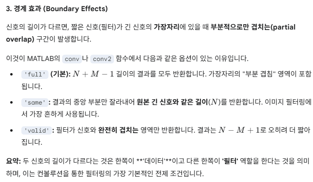
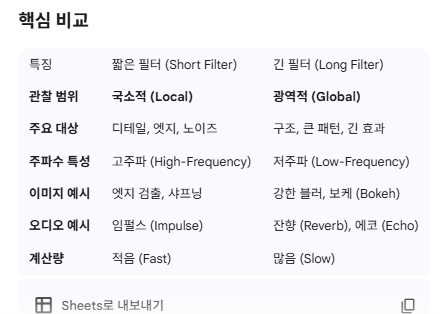
HW6
Q6.1
clear all; close all; clc;

n =[0:1:9];
x1_n = [1, 1, 1, 1, 1, 1, 1, 1, 1, 1];
x2_n = [1, 1, 1, 1, 1, -1, -1, -1, -1, -1];
x3_n = [1, 1, -1, -1, 1, 1, -1, -1, 1, 1];
x4_n = [1, -1, 1, -1, 1, -1, 1, -1, 1, -1];

k = [0:1:199];
w_k = k*2*pi/200;

X1_DTFT = sum((x1_n.').*exp(-1j * (n.' .* w_k)), 1); % X1 = x1_n*exp(-1j * (n.' .* w_k));
X2_DTFT = sum((x2_n.').*exp(-1j * (n.' .* w_k)), 1); % X2 = x2_n*exp(-1j * (n.' .* w_k));
X3_DTFT = sum((x3_n.').*exp(-1j * (n.' .* w_k)), 1); % X3 = x3_n*exp(-1j * (n.' .* w_k));
X4_DTFT = sum((x4_n.').*exp(-1j * (n.' .* w_k)), 1); % X4 = x4_n*exp(-1j * (n.' .* w_k));

axis_Pi = @(w) w/pi;

X_DTFT_Set = {X1_DTFT, X2_DTFT, X3_DTFT, X4_DTFT};
Label_Set = {'x_1','x_2','x_3','x_4'};

for i=1:4
    figure;
    Xi_DTFT = X_DTFT_Set{i};
    Label_i = Label_Set{i};

    subplot(2, 2, 1);
    plot(axis_Pi(w_k), real(Xi_DTFT)); grid on; xlim([-2 2]);
    title([Label_i ' Re']); xlabel('\omega/\pi'); ylabel('Real');

    subplot(2, 2, 2);
    plot(axis_Pi(w_k), imag(Xi_DTFT)); grid on; xlim([-2 2]);
    title([Label_i ' Im']); xlabel('\omega/\pi'); ylabel('Imag');

    subplot(2, 2, 3);
    plot(axis_Pi(w_k), abs(Xi_DTFT)); grid on; xlim([-2 2]);
    title([Label_i ' |X|']); xlabel('\omega/\pi'); ylabel('|X|');

    subplot(2, 2, 4);
    plot(axis_Pi(w_k), angle(Xi_DTFT)); grid on; xlim([-2 2]);
    title([Label_i ' \angleX']); xlabel('\omega/\pi'); ylabel('\angleX');
end
Q6.2
clear all; close all; clc;

n =[0:1:9];
x1_n = [1, 1, 1, 1, 1, 1, 1, 1, 1, 1];
x2_n = [1, 1, 1, 1, 1, -1, -1, -1, -1, -1];
x3_n = [1, 1, -1, -1, 1, 1, -1, -1, 1, 1];
x4_n = [1, -1, 1, -1, 1, -1, 1, -1, 1, -1];

k = [0:1:199];
w_k = k*2*pi/200;

X1 = sum((x1_n.').*exp(-1j * (n.' .* w_k)), 1); % X1 = x1_n*exp(-1j * (n.' .* w_k));
X2 = sum((x2_n.').*exp(-1j * (n.' .* w_k)), 1); % X2 = x2_n*exp(-1j * (n.' .* w_k));
X3 = sum((x3_n.').*exp(-1j * (n.' .* w_k)), 1); % X3 = x3_n*exp(-1j * (n.' .* w_k));
X4 = sum((x4_n.').*exp(-1j * (n.' .* w_k)), 1); % X4 = x4_n*exp(-1j * (n.' .* w_k));

axis_Pi = @(w) w/pi;

X_Set = {X1,X2,X3,X4}; Label_Set = {'x_1','x_2','x_3','x_4'};

HighFrequency = (w_k >= 0.5*pi & w_k <= 1.5*pi);

fprintf('\n=== Dominant peak frequency (argmax |X|) ===\n');
for i=1:4
    Xi = X_Set{i};
    [mx, idx] = max(abs(Xi));
    fprintf('%s: max|X| at k=%d  (ω=%.4f rad, ω/π=%.4f)\n', ...
        Label_Set{i}, idx-1, w_k(idx), w_k(idx)/pi);
end

figure;
for i=1:4
    subplot(2,2,i);
    Xi = X_Set{i};
    plot(w_k/pi, abs(Xi)); grid on; xlim([0 2]);
    xlabel('\omega/\pi'); ylabel('|X|');
    title(['|X_', Label_Set{i}, '(e^{j\omega})|']);
    [max_value, idx] = max(abs(Xi));
    hold on; xline(w_k(idx)/pi, '--');
    yl = ylim;
    area([0.8 1.2], [yl(2) yl(2)], yl(1), 'FaceAlpha', 0.05, 'EdgeColor', 'none');
end
Q6.3
clear all; close all; clc;

n =[0:1:9];
x1_n = [1, 1, 1, 1, 1, 1, 1, 1, 1, 1];
x2_n = [1, 1, 1, 1, 1, -1, -1, -1, -1, -1];
x3_n = [1, 1, -1, -1, 1, 1, -1, -1, 1, 1];
x4_n = [1, -1, 1, -1, 1, -1, 1, -1, 1, -1];

k = [0:1:399];
w_k = k*2*pi/200;

X1 = sum((x1_n.').*exp(-1j * (n.' .* w_k)), 1); % X1 = x1_n*exp(-1j * (n.' .* w_k));
X2 = sum((x2_n.').*exp(-1j * (n.' .* w_k)), 1); % X2 = x2_n*exp(-1j * (n.' .* w_k));
X3 = sum((x3_n.').*exp(-1j * (n.' .* w_k)), 1); % X3 = x3_n*exp(-1j * (n.' .* w_k));
X4 = sum((x4_n.').*exp(-1j * (n.' .* w_k)), 1); % X4 = x4_n*exp(-1j * (n.' .* w_k));

axis_Pi = @(w) w/pi;

X_Set = {X1,X2,X3,X4}; Label_Set = {'x_1','x_2','x_3','x_4'};
for i=1:4
    figure;
    Xi = X_Set{i};
    Label_i = Label_Set{i};

    subplot(2, 2, 1);
    plot(axis_Pi(w_k), real(Xi)); grid on; xlim([-2 4]);
    title([Label_i ' Re']); xlabel('\omega/\pi'); ylabel('Real');

    subplot(2, 2, 2);
    plot(axis_Pi(w_k), imag(Xi)); grid on; xlim([-2 4]);
    title([Label_i ' Im']); xlabel('\omega/\pi'); ylabel('Imag');

    subplot(2, 2, 3);
    plot(axis_Pi(w_k), abs(Xi)); grid on; xlim([-2 4]);
    title([Label_i ' |X|']); xlabel('\omega/\pi'); ylabel('|X|');

    subplot(2, 2, 4);
    plot(axis_Pi(w_k), angle(Xi)); grid on; xlim([-2 4]);
    title([Label_i ' \angleX']); xlabel('\omega/\pi'); ylabel('\angleX');
end
Q6.4
clear all; close all; clc;

n =[0:1:9];
x1_n = [1, 1, 1, 1, 1, 1, 1, 1, 1, 1];
x2_n = [1, 1, 1, 1, 1, -1, -1, -1, -1, -1];
x3_n = [1, 1, -1, -1, 1, 1, -1, -1, 1, 1];
x4_n = [1, -1, 1, -1, 1, -1, 1, -1, 1, -1];

k = [0:1:399];
w_k = k*2*pi/200;

M = 10;
m = [0:1:M-1];
w_M = 2*pi*m/M;

X1_DTFT = sum((x1_n.').*exp(-1j * (n.' .* w_k)), 1); % X1 = x1_n*exp(-1j * (n.' .* w_k));
X2_DTFT = sum((x2_n.').*exp(-1j * (n.' .* w_k)), 1); % X2 = x2_n*exp(-1j * (n.' .* w_k));
X3_DTFT = sum((x3_n.').*exp(-1j * (n.' .* w_k)), 1); % X3 = x3_n*exp(-1j * (n.' .* w_k));
X4_DTFT = sum((x4_n.').*exp(-1j * (n.' .* w_k)), 1); % X4 = x4_n*exp(-1j * (n.' .* w_k));

X1_DFT = sum((x1_n.').*exp(-1j * (n.' .* w_M)), 1); % X1 = x1_n*exp(-1j * (n.' .* w_M));
X2_DFT = sum((x2_n.').*exp(-1j * (n.' .* w_M)), 1); % X2 = x2_n*exp(-1j * (n.' .* w_M));
X3_DFT = sum((x3_n.').*exp(-1j * (n.' .* w_M)), 1); % X3 = x3_n*exp(-1j * (n.' .* w_M));
X4_DFT = sum((x4_n.').*exp(-1j * (n.' .* w_M)), 1); % X4 = x4_n*exp(-1j * (n.' .* w_M));

axis_Pi = @(w) w/pi;

X_DTFT_Set = {X1_DTFT, X2_DTFT, X3_DTFT, X4_DTFT};
X_DFT_Set = {X1_DFT, X2_DFT, X3_DFT, X4_DFT};
Label_Set = {'x_1','x_2','x_3','x_4'};

figure;
for i=1:4
    Xi_DTFT = X_DTFT_Set{i};
    Xi_DFT = X_DFT_Set{i};

    subplot(2, 2, i);
    hold on; grid on; xlim([-2 2]);
    plot(axis_Pi(w_k), abs(Xi_DTFT));
    stem(axis_Pi(w_M), abs(Xi_DFT));
    title([Label_Set{i} ' DTFT & DFT(M=10)']); xlabel('\omega/\pi'); ylabel('|X|');
    legend('DTFT (dense)','DFT samples','Location','best');
end
Q6.5
clear all; close all; clc;

n =[0:1:9];
x1_n = [1, 1, 1, 1, 1, 1, 1, 1, 1, 1];
x2_n = [1, 1, 1, 1, 1, -1, -1, -1, -1, -1];
x3_n = [1, 1, -1, -1, 1, 1, -1, -1, 1, 1];
x4_n = [1, -1, 1, -1, 1, -1, 1, -1, 1, -1];

k = [0:1:399];
w_k = k*2*pi/200;

M = 10;
m = [0:1:M-1];
w_M = 2*pi*m/M;

X1_DTFT = sum((x1_n.').*exp(-1j * (n.' .* w_k)), 1); % X1 = x1_n*exp(-1j * (n.' .* w_k));
X2_DTFT = sum((x2_n.').*exp(-1j * (n.' .* w_k)), 1); % X2 = x2_n*exp(-1j * (n.' .* w_k));
X3_DTFT = sum((x3_n.').*exp(-1j * (n.' .* w_k)), 1); % X3 = x3_n*exp(-1j * (n.' .* w_k));
X4_DTFT = sum((x4_n.').*exp(-1j * (n.' .* w_k)), 1); % X4 = x4_n*exp(-1j * (n.' .* w_k));

X1_DFT = sum((x1_n.').*exp(-1j * (n.' .* w_M)), 1); % X1 = x1_n*exp(-1j * (n.' .* w_M));
X2_DFT = sum((x2_n.').*exp(-1j * (n.' .* w_M)), 1); % X2 = x2_n*exp(-1j * (n.' .* w_M));
X3_DFT = sum((x3_n.').*exp(-1j * (n.' .* w_M)), 1); % X3 = x3_n*exp(-1j * (n.' .* w_M));
X4_DFT = sum((x4_n.').*exp(-1j * (n.' .* w_M)), 1); % X4 = x4_n*exp(-1j * (n.' .* w_M));

X1_IDFT = (1/M)*sum(X1_DFT.*exp(1j * (n.' .* w_M)), 2);
X2_IDFT = (1/M)*sum(X2_DFT.*exp(1j * (n.' .* w_M)), 2);
X3_IDFT = (1/M)*sum(X3_DFT.*exp(1j * (n.' .* w_M)), 2);
X4_IDFT = (1/M)*sum(X4_DFT.*exp(1j * (n.' .* w_M)), 2);

axis_Pi = @(w) w/pi;

X_DTFT_Set = {X1_DTFT, X2_DTFT, X3_DTFT, X4_DTFT};
X_DFT_Set = {X1_DFT, X2_DFT, X3_DFT, X4_DFT};
X_IDFT_Set = {X1_IDFT, X2_IDFT, X3_IDFT, X4_IDFT};
x_original_Set = {x1_n, x2_n, x3_n, x4_n};
Label_Set = {'x_1','x_2','x_3','x_4'};

figure;
for i=1:4
    Xi_DTFT = X_DTFT_Set{i};
    Xi_DFT = X_DFT_Set{i};
    Xi_IDFT = X_IDFT_Set{i};
    xi_original = x_original_Set{i};

    subplot(4, 3, 3*(i-1)+1);
    plot(axis_Pi(w_k), abs(Xi_DTFT));
    title([Label_Set{i} 'DTFT']);
    xlabel('\omega/\pi'); ylabel('|X|'); grid on; xlim([-2 2]);

    subplot(4, 3, 3*(i-1)+2);
    stem(axis_Pi(w_M), abs(Xi_DFT));
    title([Label_Set{i} 'DFT']);
    xlabel('\omega/\pi'); ylabel('|X|'); grid on; xlim([-2 2]);

    subplot(4, 3, 3*(i-1)+3);
    hold on; grid on;
    stem(n, xi_original, 'filled', 'DisplayName','original');
    stem(n, real(Xi_IDFT), 'DisplayName','IDFT recon');
    title([Label_Set{i} ' Time-Domain']); xlabel('n'); ylabel('amplitude');
    xlim([0 9]); legend('Location','best');

    err_inf  = norm(xi_original - real(Xi_IDFT), inf);
    err_l2   = norm(xi_original - real(Xi_IDFT));
    fprintf('%s: max|error| = %e,  L2 error = %e\n', Label_Set{i}, err_inf, err_l2);
end
Q6.6
clear all; close all; clc;

n =[0:1:9];
x1_n = [1, 1, 1, 1, 1, 1, 1, 1, 1, 1];
x2_n = [1, 1, 1, 1, 1, -1, -1, -1, -1, -1];
x3_n = [1, 1, -1, -1, 1, 1, -1, -1, 1, 1];
x4_n = [1, -1, 1, -1, 1, -1, 1, -1, 1, -1];

n10 = [0:1:9]; n20 = [0:1:19];

k = [0:1:399]; w_k = k*2*pi/200;

M = 10; m = [0:1:M-1]; w_M = 2*pi*m/M;

X1_DTFT = sum((x1_n.').*exp(-1j * (n.' .* w_k)), 1); % X1 = x1_n*exp(-1j * (n.' .* w_k));
X2_DTFT = sum((x2_n.').*exp(-1j * (n.' .* w_k)), 1); % X2 = x2_n*exp(-1j * (n.' .* w_k));
X3_DTFT = sum((x3_n.').*exp(-1j * (n.' .* w_k)), 1); % X3 = x3_n*exp(-1j * (n.' .* w_k));
X4_DTFT = sum((x4_n.').*exp(-1j * (n.' .* w_k)), 1); % X4 = x4_n*exp(-1j * (n.' .* w_k));

X1_DFT = sum((x1_n.').*exp(-1j * (n.' .* w_M)), 1); % X1 = x1_n*exp(-1j * (n.' .* w_M));
X2_DFT = sum((x2_n.').*exp(-1j * (n.' .* w_M)), 1); % X2 = x2_n*exp(-1j * (n.' .* w_M));
X3_DFT = sum((x3_n.').*exp(-1j * (n.' .* w_M)), 1); % X3 = x3_n*exp(-1j * (n.' .* w_M));
X4_DFT = sum((x4_n.').*exp(-1j * (n.' .* w_M)), 1); % X4 = x4_n*exp(-1j * (n.' .* w_M));

X1_IDFT10 = (1/M)*sum(X1_DFT.*exp(1j * (n10.' .* w_M)), 2);
X2_IDFT10 = (1/M)*sum(X2_DFT.*exp(1j * (n10.' .* w_M)), 2);
X3_IDFT10 = (1/M)*sum(X3_DFT.*exp(1j * (n10.' .* w_M)), 2);
X4_IDFT10 = (1/M)*sum(X4_DFT.*exp(1j * (n10.' .* w_M)), 2);

X1_IDFT20 = (1/M)*sum(X1_DFT.*exp(1j * (n20.' .* w_M)), 2);
X2_IDFT20 = (1/M)*sum(X2_DFT.*exp(1j * (n20.' .* w_M)), 2);
X3_IDFT20 = (1/M)*sum(X3_DFT.*exp(1j * (n20.' .* w_M)), 2);
X4_IDFT20 = (1/M)*sum(X4_DFT.*exp(1j * (n20.' .* w_M)), 2);

axis_Pi = @(w) w/pi;

X_DTFT_Set = {X1_DTFT, X2_DTFT, X3_DTFT, X4_DTFT};
X_DFT_Set = {X1_DFT, X2_DFT, X3_DFT, X4_DFT};
X_IDFT10_Set = {X1_IDFT10, X2_IDFT10, X3_IDFT10, X4_IDFT10};
X_IDFT20_Set = {X1_IDFT20, X2_IDFT20, X3_IDFT20, X4_IDFT20};
x_original_Set = {x1_n, x2_n, x3_n, x4_n};
Label_Set = {'x_1','x_2','x_3','x_4'};

figure;
for i=1:4
    Xi_DTFT = X_DTFT_Set{i}; Xi_DFT  = X_DFT_Set{i};
    xhat20  = real(X_IDFT20_Set{i});
    x10     = x_original_Set{i}(:); x20     = repmat(x10,2,1);

    subplot(4,3,3*(i-1)+1);
    plot(axis_Pi(w_k), abs(Xi_DTFT));
    title([Label_Set{i} ' DTFT']); xlabel('\omega/\pi'); ylabel('|X|');
    grid on; xlim([0 4]);

    subplot(4,3,3*(i-1)+2);
    stem(axis_Pi(w_M), abs(Xi_DFT));
    title([Label_Set{i} ' DFT (M=10)']); xlabel('\omega/\pi'); ylabel('|X|');
    grid on; xlim([0 2]);

    subplot(4,3,3*(i-1)+3);
    hold on; grid on;
    stem(n20, x20, 'DisplayName','original');
    stem(n20, xhat20, 'DisplayName','IDFT Reconstruction');
    title([Label_Set{i} ' Time-domain (n=0..19)']);
    xlabel('n'); ylabel('amplitude'); xlim([0 19]); legend('Location','best');

    err_inf = norm(x10 - xhat20(1:10), inf);
    err_L2  = norm(x10 - xhat20(1:10));
    perr = max(abs(xhat20(11:20) - xhat20(1:10)));
    fprintf('%s: Recon max|err| (n=0..9) = %e,  L2 = %e,  periodic max|x[n+10]-x[n]| = %e\n', ...
        Label_Set{i}, err_inf, err_L2, perr);
end
Q6.7
clear all; close all; clc;

% (128 128 1 27)
load mri D

Image = double(squeeze(D(:,:,1,15)));
% Image = mat2gray(Image);

S = fftshift(fft2(Image));

figure;
subplot(1,4,1);
imshow(Image,[]); title('I(x,y) (slice #15)');

subplot(1,4,2);
imshow(abs(S),[]); title('|S(k_x,k_y)| (centered)');

subplot(1,4,3);
imshow(log(1+abs(S)),[]); title('|S(k_x,k_y)| (log, centered)');

subplot(1,4,4);
imshow(angle(S),[]); title('∠S(k_x,k_y) (centered)');
Q6.8
clear all; close all; clc;

% (128 128 1 27)
load mri D

Image = double(squeeze(D(:,:,1,15)));
% Image = mat2gray(Image);

S = fftshift(fft2(Image));

[Ny, Nx] = size(Image);
kx = [-floor(Nx/2) : 1 : ceil(Nx/2)-1];
ky = [-floor(Ny/2) : 1 : ceil(Ny/2)-1];
[KX, KY] = meshgrid(kx, ky);

mask_A = mod(KX, 2) ~= 0; % x축 방향 주파수 인덱스가 홀수면, 1
S_A = S .* mask_A;
I_A = real(ifft2(ifftshift(S_A)));

mask_B = mod(KY, 2) ~= 0; % y축 방향 주파수 인덱스가 홀수면, 1
S_B = S .* mask_B;
I_B = real(ifft2(ifftshift(S_B)));

figure;
subplot(2,3,1);
imshow(log(1+abs(S)),[]); title('Original |S| (log)');

subplot(2,3,2);
imshow(mask_A,[]); title('Mask A');

subplot(2,3,3);
imshow(mask_B,[]); title('Mask B');

subplot(2,3,4);
imshow(Image,[]); title('Original I(x,y)');

subplot(2,3,5);
imshow(I_A,[]);  title('Reconstruction (even k_x = 0)');

subplot(2,3,6);
imshow(I_B,[]);  title('Reconstruction (even k_y = 0)');
Q6.9
clear all; close all; clc;

% (128 128 1 27)
load mri D

Image = double(squeeze(D(:,:,1,15)));
S = fftshift(fft2(Image));

% 주파수 좌표
[Ny, Nx] = size(Image);
% kx = -floor(Nx/2) : ceil(Nx/2)-1;
% ky = -floor(Ny/2) : ceil(Ny/2)-1;
% [KX, KY] = meshgrid(kx, ky);

% Index 좌표
cx = floor(Nx/2) + 1;        % 중앙 x 인덱스
cy = floor(Ny/2) + 1;        % 중앙 y 인덱스
Filter_N = 32;               % 중앙 정사각 영역 크기
Filter_N_half  = Filter_N/2;

mask = false(Ny, Nx);
mask(cy-Filter_N_half+1:cy+Filter_N_half, cx-Filter_N_half+1:cx+Filter_N_half) = true;

Filtered_S = S .* mask;
Filtered_I = real(ifft2(ifftshift(Filtered_S)));

figure;
subplot(2, 2, 1);
imshow(log(1+abs(S)),[]); title('|S| (log, centered)');

subplot(2, 2, 2);
imshow(log(1+abs(Filtered_S)),[]); title('|Filtered_S| (log, centered)');

subplot(2, 2, 3);
imshow(Image,[]); title('Image (original)');

subplot(2, 2, 4);
imshow(Filtered_I,[]);  title('Filtered_Image');
Q6.10
clear all; close all; clc;

% (128 128 1 27)
load mri D

Image = double(squeeze(D(:,:,1,15)));
S = fftshift(fft2(Image));

% 주파수 좌표
[Ny, Nx] = size(Image);
% kx = -floor(Nx/2) : ceil(Nx/2)-1;
% ky = -floor(Ny/2) : ceil(Ny/2)-1;
% [KX, KY] = meshgrid(kx, ky);

% Index 좌표
cx = floor(Nx/2) + 1;        % 중앙 x 인덱스
cy = floor(Ny/2) + 1;        % 중앙 y 인덱스
Filter_N = 64;               % 중앙 정사각 영역 크기
Filter_N_half  = Filter_N/2;

mask = true(Ny, Nx);
mask(cy-Filter_N_half+1:cy+Filter_N_half, cx-Filter_N_half+1:cx+Filter_N_half) = false;

Filtered_S = S .* mask;
Filtered_I = real(ifft2(ifftshift(Filtered_S)));

figure;
subplot(2, 2, 1);
imshow(log(1+abs(S)),[]); title('|S| (log, centered)');

subplot(2, 2, 2);
imshow(log(1+abs(Filtered_S)),[]); title('|Filtered_S| (log, centered)');

subplot(2, 2, 3);
imshow(Image,[]); title('Image (original)');

subplot(2, 2, 4);
imshow(Filtered_I,[]);  title('Filtered_Image');