[Python] T-pose 분석

설명

PointCloud data를 모델에게 입력했을 때, Skeleton data와 유사한 형태로 출력하도록 키넥트를 사용하여 가져온 Skeleton data를 통해 모델을 학습시킨다.

Skeleton Data

사전에 필요한 라이브러리를 import한다.

import pandas as pd
import numpy as np
import matplotlib.pyplot as plt
import torch
import torch.nn as nn
import torch.optim as optim
from torch.utils.data import DataLoader, TensorDataset
from sklearn.model_selection import train_test_split
from sklearn.preprocessing import StandardScaler
from google.colab import drive
drive.mount('/content/gdrive')

device = 'cuda' if torch.cuda.is_available() else 'cpu'

# 랜덤 시드 고정
torch.manual_seed(777)

# GPU 사용 가능일 경우 랜덤 시드 고정
if device == 'cuda':
    torch.cuda.manual_seed_all(777)

Skeleton Data를 DataFrame형태로 출력

file_path = '/TPose_Skeleton_Sample.json'

df = pd.read_json(file_path)
df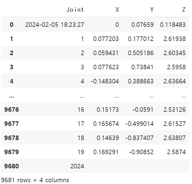

우리가 필요한 것은 X, Y, Z 좌표값이고, 마지막 행이 비어있으므로 제거

df.drop(columns=["Joint"], inplace=True)
df = df[:][:9680]
df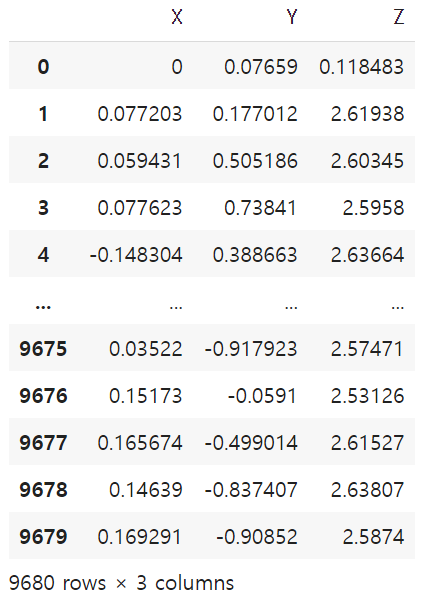

1frame 당 X, Y, Z 좌표가 각각 20개씩 나오므로 20으로 나눔

num_splits = len(df) // 20
dfs_3d = []

for i in range(num_splits):
    # 각각의 작은 DataFrame 생성
    df_split = df.iloc[i*20:(i+1)*20]

    # 작은 DataFrame을 3차원 데이터로 변환하여 리스트에 추가
    dfs_3d.append(df_split.values.reshape(20, 3, 1))

# 리스트를 NumPy 배열로 변환
data_3d = np.array(dfs_3d)

Y_data = torch.tensor(data_3d.astype(float).squeeze())

print(Y_data.shape)  # 출력: (484, 20, 3)

처음 찍힌 시간 좌표

df1 = df.loc[:19]
df1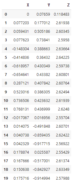

찍힌 frame의 수

len(df) / 20	# 출력: 484.0

1frame의 Skeleton Data를 3차원 그래프로 출력

fig = plt.figure()
ax = fig.add_subplot(111, projection='3d')

# 데이터프레임의 각 열을 x, y, z 좌표로 사용하여 산점도 그리기
ax.scatter(df1['X'], df1['Z'], df1['Y'], c='g')

# 축 레이블 추가
ax.set_xlabel('X Label')
ax.set_ylabel('Z Label')
ax.set_zlabel('Y Label')

plt.ylim(0,3)
plt.show()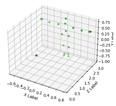

모든 frame의 Skeleton Data를 3차원 그래프로 출력

X = []
Y = []
Z = []
# 3차원 그래프 생성
fig = plt.figure()
ax = fig.add_subplot(111, projection='3d')

# 데이터를 플로팅
for i in range(len(data_3d)):
  for j in range(20):
    X.append(data_3d[i][j][0])
    Y.append(data_3d[i][j][1])
    Z.append(data_3d[i][j][2])
ax.scatter(X, Z, Y, c='g')

# 그래프 설정
ax.set_xlabel('X Label')
ax.set_ylabel('Y Label')
ax.set_zlabel('Z Label')

plt.show()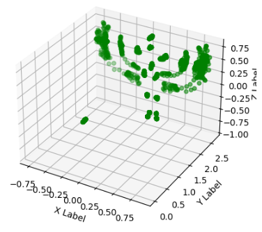

데이터 정규화

tensor_data = [torch.tensor(frame) for frame in Y_data]

scaler = StandardScaler()
for i in range(len(tensor_data)):
    frame = tensor_data[i].numpy().reshape(-1, 3)
    normalized_frame = scaler.fit_transform(frame)
    tensor_data[i] = torch.tensor(normalized_frame)

Y_data = [frame.tolist() for frame in tensor_data]

PointCloud Data

PointCloud Data를 DataFrame형태로 출력

file_path = '/TPose_pointCloud_Sample.json'

df_pc = pd.read_json(file_path, lines=True)
df_pc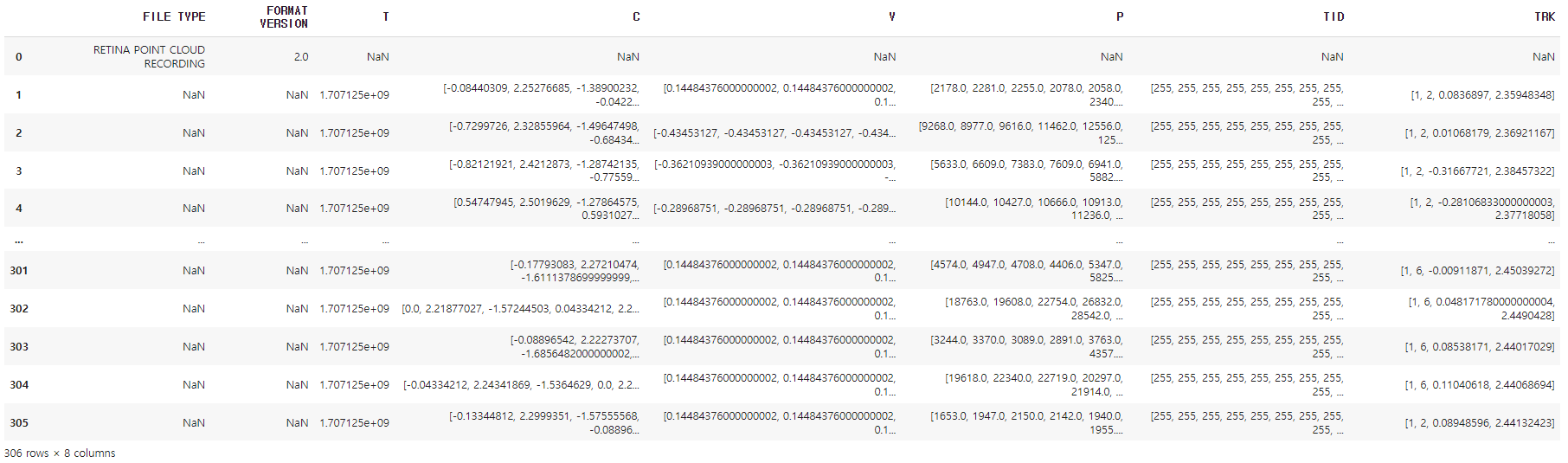

좌표값을 나타내는 행은 C이므로 나머지 행 제거

df_pc = df_pc["C"]
df_pc = df_pc[1:]
df_pc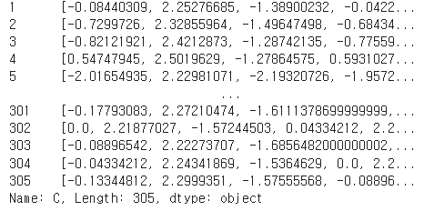

1frame의 시간 좌표

df_r = df_pc.loc[1]
df_r

PointCloud Data의 전체적인 형태

df_pc.shape	# 출력: (305, )

시각화

print('최대 길이 :',max(len(review) for review in df_pc))
print('평균 길이 :',sum(map(len, df_pc))/len(df_pc))
plt.hist([len(review) for review in df_pc], bins=50)
plt.xlabel('length of samples')
plt.ylabel('number of samples')
plt.show()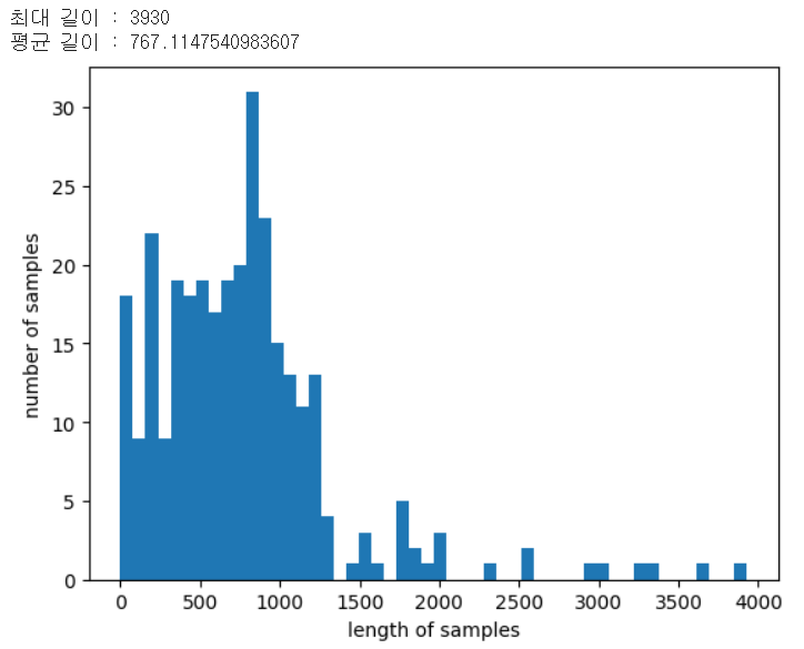

분포도 계산

def below_threshold_len(max_len, nested_list):
  count = 0
  for sentence in nested_list:
    if(len(sentence) <= max_len):
        count = count + 1
  print('전체 샘플 중 길이가 %s 이하인 샘플의 비율: %s'%(max_len, (count / len(nested_list))*100))
  
max_len = 1500
below_threshold_len(max_len, df_pc)

frame 마다 좌표의 개수가 다르므로 패딩을 통해서 같게 만들어줌

패딩 함수

def pad_sequences(sentences, max_len):
  features = np.zeros((len(sentences), max_len), dtype=float)
  for index, sentence in enumerate(sentences):
    if len(sentence) != 0:
      features[index, :len(sentence)] = np.array(sentence)[:max_len]
  return features

패딩 결과 확인

padded_data = pad_sequences(df_pc, 1500)
len(padded_data[1])

PointCloud Data를 X, Y, Z 좌표로 나눔

X = []
Y = []
Z = []
new = {"X":[], "Y":[], "Z":[]}

for i in range(len(df_r)):
  if i % 3 == 0:
    X.append(df_r[i])
  elif i % 3 == 1:
    Z.append(df_r[i])
  else:
    Y.append(df_r[i])
new["X"] = X
new["Y"] = Y
new["Z"] = Z
pointcloud = pd.DataFrame(new)
pointcloud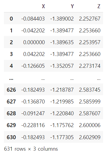

1frame의 PointCloud Data 3차원 그래프로 출력

fig = plt.figure()
ax = fig.add_subplot(111, projection='3d')

# 데이터프레임의 각 열을 x, y, z 좌표로 사용하여 산점도 그리기
ax.scatter(pointcloud['X'], pointcloud['Z'], pointcloud['Y'], c='g')

# 축 레이블 추가
ax.set_xlabel('X Label')
ax.set_ylabel('Z Label')
ax.set_zlabel('Y Label')

plt.ylim(0,3)
plt.show()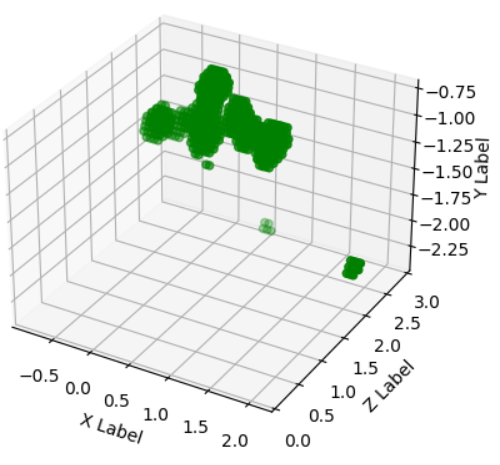

모든 frame의 데이터를 X, Y, Z 좌표로 분할

X = []
Y = []
Z = []
new = {"X":[], "Y":[], "Z":[]}

for i in range(len(padded_data)):
  for j in range(len(padded_data[i])):
    if j % 3 == 0:
      X.append(padded_data[i][j])
    elif j % 3 == 1:
      Z.append(padded_data[i][j])
    else:
      Y.append(padded_data[i][j])
new["X"] = X
new["Y"] = Y
new["Z"] = Z

X_data = pd.DataFrame(new)

데이터 차원 조절

num_splits = len(X_data) // 500
dfs_3dd = []

for i in range(num_splits):
    # 각각의 작은 DataFrame 생성
    df_split = X_data.iloc[i*500:(i+1)*500]

    # 작은 DataFrame을 3차원 데이터로 변환하여 리스트에 추가
    dfs_3dd.append(df_split.values.reshape(500, 3, 1))

# 리스트를 NumPy 배열로 변환
data_3dd = np.array(dfs_3dd)

# PointCloud data
X_data = data_3dd.astype(float).squeeze()
X_data.shape

print(X_data.shape)	# 출력 (305, 500, 3)

데이터 정규화

tensor_data = [torch.tensor(frame) for frame in X_data]

scaler = StandardScaler()
for i in range(len(tensor_data)):
    frame = tensor_data[i].numpy().reshape(-1, 3)
    normalized_frame = scaler.fit_transform(frame)
    tensor_data[i] = torch.tensor(normalized_frame)

X_data = [frame.tolist() for frame in tensor_data]

모델

훈련셋과 검증셋 구분

X_train, X_test, y_train, y_test = train_test_split(X_data, Y_data, test_size= 0.2, random_state=1234)

pytorch가 원하는 데이터 구조로 변경

X_train = np.transpose(X_train, (0, 2, 1))
X_test = np.transpose(X_test, (0, 2, 1))
y_train = np.transpose(y_train, (0, 2, 1))
y_test = np.transpose(y_test, (0, 2, 1))

Tensor로 변환

tensor_X_train = torch.tensor(X_train).float() # torch.Size([244, 3, 500]) 
tensor_X_test = torch.tensor(X_test).float() # torch.Size([61, 3, 500])
tensor_y_train = torch.tensor(y_train).float() # torch.Size([244, 3, 20])
tensor_y_test = torch.tensor(y_test).float() # torch.Size([61, 3, 20])

Dataset, DataLoader 설정

train_dataset = TensorDataset(tensor_X_train, tensor_y_train)
test_dataset = TensorDataset(tensor_X_test, tensor_y_test)

train_loader = DataLoader(dataset=train_dataset, batch_size=3, shuffle=True)
test_loader = DataLoader(test_dataset, batch_size=3, shuffle=False)

learning_rate = 0.001
training_epochs = 50

CNN 모델 정의

class CNN(nn.Module):
    def __init__(self):
        super(CNN, self).__init__()
        # input=3, output=64
        self.layer1 = nn.Sequential(
            nn.Conv1d(3, 64, kernel_size=3, stride=1, padding=1),
            nn.ReLU(),
            nn.MaxPool1d(2))
		
        # input=64, output=15
        self.layer2 = nn.Sequential(
            nn.Conv1d(64, 15, kernel_size=3, stride=1, padding=1),
            nn.ReLU(),
            nn.MaxPool1d(2))

        self.fc1 = nn.Linear(15 * 125, 3 * 20)

    def forward(self, x):
        out = self.layer1(x)
        out = self.layer2(out)
        out = out.view(out.size(0), -1)
        out = self.fc1(out)
        return out

모델 학습

# 모델 생성
model = CNN().to(device)

criterion = torch.nn.MSELoss()
optimizer = torch.optim.Adam(model.parameters(), lr=learning_rate)

for epoch in range(training_epochs):
    running_loss = 0.0
    for X, Y in train_loader:
        X_train = X.to(device)
        Y_train = Y.to(device)
        optimizer.zero_grad()
        hypothesis = model(X_train)
        loss = criterion(hypothesis, Y_train.view(Y_train.size(0), -1))
        loss.backward()
        optimizer.step()
        running_loss += loss.item()

    print(f'Epoch [{epoch + 1}/{training_epochs}], Loss: {running_loss / len(train_loader):.4f}')

print('Finished Training')

모델 평가

model.eval()

with torch.no_grad():
  X_test = tensor_X_test.to(device)
  Y_test = tensor_y_test.to(device)
  test_outputs = model(X_test)
  test_loss = criterion(test_outputs, Y_test.reshape(Y_test.size(0), -1))
  print(f'Test Loss: {test_loss.item():.4f}')

output reshape

output = test_outputs.reshape(61, 3, 20)

output data 3차원 그래프로 출력

X = []
Y = []
Z = []
# 3차원 그래프 생성
fig = plt.figure()
ax = fig.add_subplot(111, projection='3d')

# 데이터를 플로팅
for i in range(len(dd)):
  for j in range(20):
    X.append(dd[i][0][j].cpu().numpy())
    Y.append(dd[i][1][j].cpu().numpy())
    Z.append(dd[i][2][j].cpu().numpy())
ax.scatter(X, Z, Y, c='g')

# 그래프 설정
ax.set_xlabel('X Label')
ax.set_ylabel('Z Label')
ax.set_zlabel('Y Label')

plt.show()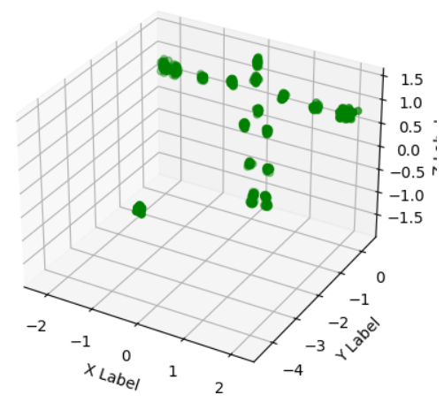