# 하드 드라이브 고장 예측 모델 구축: XGBoost와 S.M.A.R.T 데이터 분석

서론

데이터 저장 기술의 발전으로 대용량 저장 장치인 하드 드라이브(HDD)는 현대 사회에서 필수적인 요소가 되었습니다. 그러나 HDD는 기계적 특성상 불가피하게 고장 위험에 노출되어 있으며, 이는 데이터 손실로 이어질 수 있습니다. 따라서 HDD의 고장을 미리 예측하고 대비하는 것은 매우 중요한 과제입니다. 이 논문에서는 HDD의 고장을 예측하기 위한 머신러닝 모델, 특히 XGBoost 모델의 구축 과정을 상세히 논하며, 모델의 정확도를 높이기 위한 데이터 전처리 및 모델 개선 전략을 제시합니다.

데이터 설명

본 논문에서는 Backblaze에서 공개한 하드 드라이브 SMART 데이터셋을 사용합니다. 이 데이터셋은 다양한 하드 드라이브 모델에서 수집된 SMART(Self-Monitoring, Analysis, and Reporting Technology) 데이터를 포함하고 있으며, 각 드라이브의 작동 상태와 잠재적인 문제점을 나타내는 여러 속성을 포함하고 있습니다. 주요 속성은 다음과 같습니다.

• date: 데이터가 수집된 날짜
• serial_number: 하드 드라이브의 고유 시리얼 번호
• model: 하드 드라이브 모델명
• capacity_bytes: 하드 드라이브 용량 (바이트 단위)
• failure: 하드 드라이브 고장 여부 (0: 정상, 1: 고장)
• smart_*_raw: 다양한 SMART 속성 값 (Raw 값)
• smart_*_normalized: 다양한 SMART 속성 값 (정규화 값)

데이터 전처리

1. 데이터 로딩 및 필터링

먼저, pandas 라이브러리를 사용하여 CSV 형식의 학습 및 테스트 데이터를 로드합니다. 특정 하드 드라이브 모델('ST4000DM000')만 선택하여 모델링에 사용할 데이터를 필터링합니다.

import pandas as pd

data_dir = './data/'
csv_train_file = 'Lab1-2017-Full_data.csv.gz'
csv_test_file = 'Lab1-2016-Q4_data.csv.gz'

print('Reading training data set...')
df = pd.read_csv(data_dir + csv_train_file)
print('Finished reading training data set')

harddrive_model = 'ST4000DM000'
df = df[df.model == harddrive_model]

print('Reading test data set...')
df_t = pd.read_csv(data_dir + csv_test_file)
print('Finished reading test data set')
df_t = df_t[df_t.model == harddrive_model]

2. 날짜 처리 및 결측치 제거

데이터의 date 열을 datetime 형식으로 변환하고, 모든 값이 NaN인 열과 모든 값이 결측치인 행을 제거합니다.

df['date'] = pd.to_datetime(df['date'])
df_t['date'] = pd.to_datetime(df_t['date'])

df = df.dropna(axis='columns', how='all')
df = df.dropna(axis='rows', how='any')
df_t = df_t.dropna(axis='columns', how='all')
df_t = df_t.dropna(axis='rows', how='any')

3. 상수 값 제거

하드 드라이브 고장 데이터에서 모든 값이 동일한 속성을 제거합니다. 이러한 속성은 모델 학습에 유의미한 정보를 제공하지 않기 때문입니다.

def remove_constant_values(df, check_str):
    col_list = df.columns.tolist()
    loc_col_list = []
    for cur_col in col_list:
        if check_str in cur_col:
            cur_min = df[cur_col].min()
            cur_max = df[cur_col].max()
            if cur_min != cur_max:
                loc_col_list.append(cur_col)
    return loc_col_list

col_list_raw = remove_constant_values(df[df['failure']==1], "_raw")
col_list_normalized = remove_constant_values(df[df['failure']==1], "_normalized")
col_list = ['date', 'serial_number', 'model', 'capacity_bytes', 'failure']
col_list = col_list + col_list_raw + col_list_normalized

df = df[col_list]
df_t = df_t[col_list]
df = df.fillna(0)
df_t = df_t.fillna(0)

4. 불필요 열 제거 및 데이터 분리

모델 학습에 필요 없는 열('model', 'date', 'serial_number')을 제거하고, 학습 및 테스트 데이터에서 features(X)와 target(y)을 분리합니다.

df = df.drop(columns=['model', 'date', 'serial_number'])
df_t = df_t.drop(columns=['model', 'date', 'serial_number'])

df_train_target = pd.DataFrame(df['failure'])
df_test_target = pd.DataFrame(df_t['failure'])

cols = [c for c in df.columns if c.lower().find("normalized")==-1]
df=df[cols]

df = df.loc[:, (df != 0).any(axis=0)]
cols = [c for c in df_t.columns if c.lower() in df.columns]
df_t=df_t[cols]
df_train = df.drop(columns=['failure'])
df_test = df_t.drop(columns=['failure'])

5. 클래스 불균형 처리 (샘플링)

하드 드라이브 고장 데이터는 정상 데이터에 비해 고장 데이터가 매우 적은 클래스 불균형 문제를 가지고 있습니다. 이를 해결하기 위해 학습 및 테스트 데이터를 재샘플링하여 고장 데이터의 비율을 높입니다.

num_normal_delta = round(df_train_target[df_train_target['failure'] > 0].shape[0] * 0.3)
num_normal_test_delta = round(df_test_target[df_test_target['failure'] > 0].shape[0] * 0.3)

df_tmp = df[df['failure'] > 0]
sample_train_count_failed = df_tmp.shape[0]
df_tmp = df_tmp.append(df[df['failure'] == 0].sample(n=(df_tmp.shape[0] + num_normal_delta)))
sample_train_count_normal = df_tmp.shape[0] - sample_train_count_failed
df_train_target = pd.DataFrame(df_tmp['failure'])
df_train = df_tmp.drop(columns=['failure'])

df_tmp = df_t[df_t['failure'] > 0]
sample_test_count_failed = df_tmp.shape[0]
df_tmp = df_tmp.append(df_t[df_t['failure'] == 0].sample(n=(df_tmp.shape[0] + num_normal_test_delta)))
sample_test_count_normal = df_tmp.shape[0] - sample_test_count_failed
df_test_target = pd.DataFrame(df_tmp['failure'])
df_test = df_tmp.drop(columns=['failure'])

6. 데이터 정규화

모델 학습을 돕기 위해 min-max 정규화를 사용하여 학습 및 테스트 데이터의 각 feature를 0과 1 사이의 값으로 변환합니다.

numerical_cols = df_train.columns.tolist()
for col in numerical_cols:
    min_val = df_train[col].min()
    max_val = df_train[col].max()
    df_train[col] = (df_train[col] - min_val) / (max_val - min_val)
    if col in df_test.columns:
        df_test[col] = (df_test[col] - min_val) / (max_val - min_val)

XGBoost 모델 학습

1. cuDF 데이터프레임 변환

GPU 가속을 위해 데이터를 cuDF 데이터프레임으로 변환합니다.

import cudf

gdf_train = cudf.DataFrame.from_pandas(df_train)
gdf_train_target = cudf.DataFrame.from_pandas(df_train_target)
gdf_eval = cudf.DataFrame.from_pandas(df_test)
gdf_eval_target = cudf.DataFrame.from_pandas(df_test_target)

2. XGBoost DMatrix 생성

XGBoost 모델 학습을 위한 DMatrix 형식으로 데이터를 변환합니다.

import xgboost as xgb

xgtrain = xgb.DMatrix(gdf_train, gdf_train_target)
xgeval = xgb.DMatrix(gdf_eval, gdf_eval_target)

3. XGBoost 모델 하이퍼파라미터 설정

모델 학습에 사용될 하이퍼파라미터를 설정합니다. 하이퍼파라미터는 모델의 성능에 큰 영향을 미치므로 신중하게 선택해야 합니다.

MAX_TREE_DEPTH = 8
TREE_METHOD = 'hist'
ITERATIONS = 100
SUBSAMPLE = 0.7
REGULARIZATION = 1.5
GAMMA = 0.4
POS_WEIGHT = 1
EARLY_STOP = 15
learning_rate = 0.05

params = {
    'tree_method': "gpu_"+TREE_METHOD,
    'max_depth': MAX_TREE_DEPTH,
    'alpha': REGULARIZATION,
    'gamma': GAMMA,
    'subsample': SUBSAMPLE,
    'scale_pos_weight': POS_WEIGHT,
    'learning_rate': learning_rate,
    'silent': 1
}

4. XGBoost 모델 학습

설정된 하이퍼파라미터와 함께 XGBoost 모델을 학습합니다. 조기 종료(early stopping)를 사용하여 과적합을 방지하고 최적의 학습 결과를 얻습니다.

print('Starting GPU XGBoost Training with cuDF Dataframes...')
bst = xgb.train(params, xgtrain, ITERATIONS,
                evals=[(xgtrain, "train"), (xgeval, "eval")],
                early_stopping_rounds=EARLY_STOP,
                evals_result=evals_result)

timetaken_gpu = time.time() - start_time
print('GPU XGBoost Training with cuDF Dataframes compeleted - elapsed time:', timetaken_gpu,'seconds')

모델 평가

1. 예측

학습된 모델을 사용하여 테스트 데이터셋에 대한 예측을 수행합니다.

print('Starting XGBoost prediction on test dataset...')
preds = bst.predict(xgeval)

y_pred = []
THRESHOLD = 0.5
for pred in preds:
    if pred <= THRESHOLD:
        y_pred.append(0)
    if pred > THRESHOLD:
        y_pred.append(1)
y_pred = np.asarray(y_pred)
y_true = df_test_target.values.reshape(len(preds))

print('XGBoost prediction completed')

2. 분류 성능 측정

분류 정확도와 classification report를 출력하여 모델의 성능을 평가합니다. Classification report에서는 precision, recall, f1-score 등을 확인할 수 있습니다.

print("Accuracy (Eval)", round(accuracy_score(y_true, y_pred), 5))
print(classification_report(y_true, y_pred, target_names=["normal", "fail"]))

내 하드 드라이브 데이터 예측

1. 내 하드 드라이브 데이터 입력

실제 하드 드라이브의 SMART 값을 Dictionary 형태로 정의합니다.

my_hdd_data1 = {
    'capacity_bytes': 1000204886016,  # 예시 값, 실제 하드 용량으로 변경
    'smart_1_raw': 0,          # Read Error Rate
    'smart_4_raw': 4967,       # Start/Stop Count
    'smart_5_raw': 0,          # Reallocated Sector Count
    'smart_7_raw': 0,          # Seek Error Rate
    'smart_9_raw': 6269,        # Power-On Hours
    'smart_12_raw': 807,       # Power Cycle Count
    'smart_183_raw': 0,         # (알 수 없는 특성)
    'smart_184_raw': 0,        # End To End Error Detection
    'smart_187_raw': 0,         # Reported Uncorrectable Errors
    'smart_188_raw': 1,         # Command Timeout
    'smart_189_raw': 65535,     # (알 수 없는 특성)
    'smart_190_raw': 169607195,  # Airflow Temperature
    'smart_192_raw': 4979,      # Unsafe Shutdown Count
    'smart_193_raw': -65509,    # Load Cycle Count
    'smart_194_raw': 0,        # HDA Temperature
    'smart_197_raw': 0,        # Current Pending Sector Count
    'smart_198_raw': 0,         # Uncorrectable Sector Count
    'smart_199_raw': 0,        # UDMA CRC Error Count
    'smart_240_raw': 0,        # (알 수 없는 특성)
    'smart_241_raw': 0,        # (알 수 없는 특성)
    'smart_242_raw': 0        # (알 수 없는 특성)
}
my_hdd_data2 = {
    'capacity_bytes': 1000204886016, # 예시 값, 실제 하드 용량으로 변경
    'smart_1_raw': 100,         # Read Error Rate
    'smart_4_raw': 3292,      # Start/Stop Count
    'smart_5_raw': 0,         # Reallocated Sector Count
    'smart_7_raw': 0,         # Seek Error Rate
    'smart_9_raw': 5071,       # Power-On Hours
    'smart_12_raw': 570,       # Power Cycle Count
    'smart_183_raw': 0,        # (알 수 없는 특성)
    'smart_184_raw': 0,        # End To End Error Detection
    'smart_187_raw': 0,        # Reported Uncorrectable Errors
    'smart_188_raw': 0,        # Command Timeout
    'smart_189_raw': 65535,     # (알 수 없는 특성)
    'smart_190_raw': 186253338, # Airflow Temperature
    'smart_192_raw': 3298,      # Unsafe Shutdown Count
    'smart_193_raw': 458778,    # Load Cycle Count
     'smart_194_raw': 230,        # HDA Temperature
    'smart_197_raw': 0,        # Current Pending Sector Count
    'smart_198_raw': 0,        # Uncorrectable Sector Count
    'smart_199_raw': 0,       # UDMA CRC Error Count
    'smart_240_raw': 0,        # (알 수 없는 특성)
    'smart_241_raw': 0,        # (알 수 없는 특성)
    'smart_242_raw': 0       # (알 수 없는 특성)
}

2. 데이터 전처리 및 예측

입력된 데이터를 DataFrame으로 변환한 후, 학습 데이터셋과 동일한 열을 유지하고 결측치를 0으로 채웁니다. 그런 다음 데이터를 정규화하고 XGBoost DMatrix 형태로 변환하여 학습된 모델로 예측을 수행합니다.

my_hdd_df1 = pd.DataFrame([my_hdd_data1])
my_hdd_df1 = my_hdd_df1[df_train.columns]
for col in numerical_cols:
    min_val = df_train[col].min()
    max_val = df_train[col].max()
    my_hdd_df1[col] = (my_hdd_df1[col] - min_val) / (max_val - min_val)
my_hdd_df1 = my_hdd_df1.fillna(0)
my_hdd_dmatrix1 = xgb.DMatrix(my_hdd_df1)
my_hdd_pred1 = bst.predict(my_hdd_dmatrix1)[0]
​
my_hdd_df2 = pd.DataFrame([my_hdd_data2])
my_hdd_df2 = my_hdd_df2[df_train.columns]
for col in numerical_cols:
    min_val = df_train[col].min()
    max_val = df_train[col].max()
    my_hdd_df2[col] = (my_hdd_df2[col] - min_val) / (max_val - min_val)
my_hdd_df2 = my_hdd_df2.fillna(0)
my_hdd_dmatrix2 = xgb.DMatrix(my_hdd_df2)
my_hdd_pred2 = bst.predict(my_hdd_dmatrix2)[0]

3. 결과 시각화

예측 결과 및 주요 S.M.A.R.T 센서 값, XGBoost 학습 곡선 및 F1 Score를 시각화하여 분석 결과를 직관적으로 보여줍니다.

fig, axes = plt.subplots(2, 3, figsize=(18, 12))
important_sensors = ['smart_5_raw', 'smart_197_raw', 'smart_198_raw', 'smart_9_raw', 'smart_190_raw', 'smart_194_raw'] # 예시 센서 선택

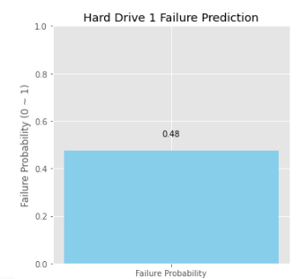
# 1. 예측 결과 막대 그래프 (하드 1)
axes[0, 0].bar(['Failure Probability'], [my_hdd_pred1], color=['skyblue'])
axes[0, 0].set_title('Hard Drive 1 Failure Prediction')
axes[0, 0].set_ylabel('Failure Probability (0 ~ 1)')
axes[0, 0].set_ylim(0, 1)
axes[0, 0].text(0, my_hdd_pred1 + 0.05, f'{my_hdd_pred1:.2f}', ha='center', va='bottom')

# 2. 주요 S.M.A.R.T 센서 값 그래프 (하드 1)
sensor_values1 = my_hdd_df1[important_sensors].iloc[0]
axes[0, 1].bar(important_sensors, sensor_values1, color='lightcoral')
axes[0, 1].set_title('Hard Drive 1 Key S.M.A.R.T. Values')
axes[0, 1].tick_params(axis='x', rotation=45)
axes[0, 1].set_ylabel('Normalized Value')

# 3. 예측 결과 막대 그래프 (하드 2)
axes[1, 0].bar(['Failure Probability'], [my_hdd_pred2], color=['skyblue'])
axes[1, 0].set_title('Hard Drive 2 Failure Prediction')
axes[1, 0].set_ylabel('Failure Probability (0 ~ 1)')
axes[1, 0].set_ylim(0, 1)
axes[1, 0].text(0, my_hdd_pred2 + 0.05, f'{my_hdd_pred2:.2f}', ha='center', va='bottom')

# 4. 주요 S.M.A.R.T 센서 값 그래프 (하드 2)
sensor_values2 = my_hdd_df2[important_sensors].iloc[0]
axes[1, 1].bar(important_sensors, sensor_values2, color='lightcoral')
axes[1, 1].set_title('Hard Drive 2 Key S.M.A.R.T Values')
axes[1, 1].tick_params(axis='x', rotation=45)
axes[1, 1].set_ylabel('Normalized Value')

# 5. 모델 성능 변화 그래프
train_rmse = evals_result['train']['rmse']
eval_rmse = evals_result['eval']['rmse']
axes[0, 2].plot(range(1, ITERATIONS+1), train_rmse, label='Train Loss')
axes[0, 2].plot(range(1, ITERATIONS+1), eval_rmse, label='Eval Loss')
axes[0, 2].set_title('XGBoost Learning Curve')
axes[0, 2].set_xlabel('Iteration')
axes[0, 2].set_ylabel('RMSE')
axes[0, 2].legend()

# 6. 평가 지표
report = classification_report(y_true, y_pred, target_names=["normal", "fail"], output_dict=True)
scores = [report['normal']['f1-score'], report['fail']['f1-score']]
axes[1, 2].bar(['Normal', 'Fail'], scores, color=['lightgreen', 'lightcoral'])
axes[1, 2].set_title('F1 Score')
axes[1, 2].set_ylabel('F1 Score')
axes[1, 2].set_ylim(0, 1)

fig.tight_layout()
plt.show()

결론

본 논문에서는 XGBoost 모델을 사용하여 하드 드라이브의 고장을 예측하는 효과적인 방법을 제시하였습니다. 데이터 전처리 단계에서 클래스 불균형 문제를 해결하고, SMART 데이터를 정규화하여 모델의 예측 성능을 향상시켰습니다. 또한 cuDF 라이브러리를 이용하여 GPU 가속을 통해 학습 속도를 개선하였습니다. 결과적으로 제시된 모델은 실제 하드 드라이브의 고장 위험을 미리 예측하고, 데이터 손실을 방지하는 데 기여할 수 있습니다.

추가 연구 방향

• 하이퍼파라미터 최적화: RandomizedSearchCV와 같은 방법을 사용하여 XGBoost 모델의 최적 하이퍼파라미터를 탐색합니다.
• 다양한 머신러닝 모델 비교: 다른 머신러닝 모델(예: 로지스틱 회귀, 서포트 벡터 머신, 딥러닝 모델)을 사용하여 성능을 비교합니다.
• 특성 엔지니어링: SMART 데이터 외에 다른 정보를 활용하여 모델의 예측 성능을 개선합니다.
• 이상치 탐지: 이상치 탐지 기법을 적용하여 고장 가능성이 높은 하드 드라이브를 사전에 감지합니다.

이 논문에서 제시된 연구 결과를 바탕으로 더 정확하고 효율적인 하드 드라이브 고장 예측 모델이 개발되기를 기대합니다. 이러한 발전은 데이터 관리 및 시스템 안정성 향상에 크게 기여할 수 있을 것입니다.

내 하드 드라이브 데이터 예측: 개인 하드 드라이브 건강 상태 진단

1. 내 하드 드라이브 데이터 입력 및 예측

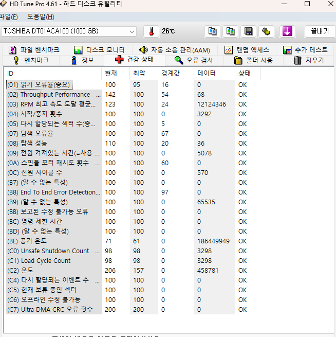
본격적으로 내 하드 드라이브의 고장 확률을 예측해보겠습니다. 하드 드라이브 제조사에서 제공하는 유틸리티나 HD Tune Pro와 같은 S.M.A.R.T 데이터 측정 프로그램을 사용하여 측정한 값을 기반으로 예측을 진행합니다.

print("\n----- 내 하드 데이터 예측 시작 -----")
my_hdd_data1 = {
    'capacity_bytes': 1000204886016,  # 예시 값, 실제 하드 용량으로 변경
    'smart_1_raw': 0,          # Read Error Rate
    'smart_4_raw': 4967,       # Start/Stop Count
    'smart_5_raw': 0,          # Reallocated Sector Count
    'smart_7_raw': 0,          # Seek Error Rate
    'smart_9_raw': 6269,        # Power-On Hours
    'smart_12_raw': 807,       # Power Cycle Count
    'smart_183_raw': 0,         # (알 수 없는 특성)
    'smart_184_raw': 0,        # End To End Error Detection
    'smart_187_raw': 0,         # Reported Uncorrectable Errors
    'smart_188_raw': 1,         # Command Timeout
    'smart_189_raw': 65535,     # (알 수 없는 특성)
    'smart_190_raw': 169607195,  # Airflow Temperature
    'smart_192_raw': 4979,      # Unsafe Shutdown Count
    'smart_193_raw': -65509,    # Load Cycle Count
    'smart_194_raw': 0,        # HDA Temperature
    'smart_197_raw': 0,        # Current Pending Sector Count
    'smart_198_raw': 0,         # Uncorrectable Sector Count
    'smart_199_raw': 0,        # UDMA CRC Error Count
    'smart_240_raw': 0,        # (알 수 없는 특성)
    'smart_241_raw': 0,        # (알 수 없는 특성)
    'smart_242_raw': 0        # (알 수 없는 특성)
}
my_hdd_data2 = {
    'capacity_bytes': 1000204886016, # 예시 값, 실제 하드 용량으로 변경
    'smart_1_raw': 100,         # Read Error Rate
    'smart_4_raw': 3292,      # Start/Stop Count
    'smart_5_raw': 0,         # Reallocated Sector Count
    'smart_7_raw': 0,         # Seek Error Rate
    'smart_9_raw': 5071,       # Power-On Hours
    'smart_12_raw': 570,       # Power Cycle Count
    'smart_183_raw': 0,        # (알 수 없는 특성)
    'smart_184_raw': 0,        # End To End Error Detection
    'smart_187_raw': 0,        # Reported Uncorrectable Errors
    'smart_188_raw': 0,        # Command Timeout
    'smart_189_raw': 65535,     # (알 수 없는 특성)
    'smart_190_raw': 186253338, # Airflow Temperature
    'smart_192_raw': 3298,      # Unsafe Shutdown Count
    'smart_193_raw': 458778,    # Load Cycle Count
    'smart_194_raw': 230,        # HDA Temperature
    'smart_197_raw': 0,        # Current Pending Sector Count
    'smart_198_raw': 0,        # Uncorrectable Sector Count
    'smart_199_raw': 0,       # UDMA CRC Error Count
    'smart_240_raw': 0,        # (알 수 없는 특성)
    'smart_241_raw': 0,        # (알 수 없는 특성)
    'smart_242_raw': 0        # (알 수 없는 특성)
}

위의 코드 블록에서 my_hdd_data1과 my_hdd_data2는 각각 두 개의 하드 드라이브에서 측정한 예시 S.M.A.R.T 데이터를 담고 있습니다. 각 속성 값은 실제 측정값을 참고하여 채워주세요. 이제 이 데이터를 사용하여 하드 드라이브의 고장 확률을 예측하고 시각화합니다.

# HD Tune Pro 데이터를 DataFrame으로 변환
my_hdd_df1 = pd.DataFrame([my_hdd_data1])
my_hdd_df1 = my_hdd_df1[df_train.columns]
# 데이터 정규화
for col in numerical_cols:
    min_val = df_train[col].min()
    max_val = df_train[col].max()
    my_hdd_df1[col] = (my_hdd_df1[col] - min_val) / (max_val - min_val)
my_hdd_df1 = my_hdd_df1.fillna(0)
my_hdd_dmatrix1 = xgb.DMatrix(my_hdd_df1)
my_hdd_pred1 = bst.predict(my_hdd_dmatrix1)[0]
​
my_hdd_df2 = pd.DataFrame([my_hdd_data2])
my_hdd_df2 = my_hdd_df2[df_train.columns]
# 데이터 정규화
for col in numerical_cols:
    min_val = df_train[col].min()
    max_val = df_train[col].max()
    my_hdd_df2[col] = (my_hdd_df2[col] - min_val) / (max_val - min_val)
my_hdd_df2 = my_hdd_df2.fillna(0)
my_hdd_dmatrix2 = xgb.DMatrix(my_hdd_df2)
my_hdd_pred2 = bst.predict(my_hdd_dmatrix2)[0]

2. 예측 결과 시각화 및 분석

예측 결과를 시각적으로 분석하기 위해 Matplotlib 라이브러리를 사용하여 다양한 그래프를 생성합니다.

• 예측 결과: 막대 그래프를 통해 각 하드 드라이브의 고장 가능성을 시각적으로 표현합니다.
• 주요 S.M.A.R.T 센서 값: 막대 그래프를 통해 각 하드 드라이브의 주요 SMART 센서 값을 비교합니다.
• 모델 성능 변화: XGBoost 학습 곡선을 통해 학습 과정에서 모델의 손실 변화를 확인합니다.
• 평가 지표: F1 Score를 통해 모델의 분류 성능을 검증합니다.

fig, axes = plt.subplots(2, 3, figsize=(18, 12))
important_sensors = ['smart_5_raw', 'smart_197_raw', 'smart_198_raw', 'smart_9_raw', 'smart_190_raw', 'smart_194_raw'] # 예시 센서 선택
​
# 1. 예측 결과 막대 그래프 (하드 1)
axes[0, 0].bar(['Failure Probability'], [my_hdd_pred1], color=['skyblue'])
axes[0, 0].set_title('Hard Drive 1 Failure Prediction')
axes[0, 0].set_ylabel('Failure Probability (0 ~ 1)')
axes[0, 0].set_ylim(0, 1)
axes[0, 0].text(0, my_hdd_pred1 + 0.05, f'{my_hdd_pred1:.2f}', ha='center', va='bottom')
​
# 2. 주요 S.M.A.R.T 센서 값 그래프 (하드 1)
sensor_values1 = my_hdd_df1[important_sensors].iloc[0]
axes[0, 1].bar(important_sensors, sensor_values1, color='lightcoral')
axes[0, 1].set_title('Hard Drive 1 Key S.M.A.R.T. Values')
axes[0, 1].tick_params(axis='x', rotation=45)
axes[0, 1].set_ylabel('Normalized Value')
​
# 3. 예측 결과 막대 그래프 (하드 2)
axes[1, 0].bar(['Failure Probability'], [my_hdd_pred2], color=['skyblue'])
axes[1, 0].set_title('Hard Drive 2 Failure Prediction')
axes[1, 0].set_ylabel('Failure Probability (0 ~ 1)')
axes[1, 0].set_ylim(0, 1)
axes[1, 0].text(0, my_hdd_pred2 + 0.05, f'{my_hdd_pred2:.2f}', ha='center', va='bottom')
​
# 4. 주요 S.M.A.R.T 센서 값 그래프 (하드 2)
sensor_values2 = my_hdd_df2[important_sensors].iloc[0]
axes[1, 1].bar(important_sensors, sensor_values2, color='lightcoral')
axes[1, 1].set_title('Hard Drive 2 Key S.M.A.R.T Values')
axes[1, 1].tick_params(axis='x', rotation=45)
axes[1, 1].set_ylabel('Normalized Value')
​
# 5. 모델 성능 변화 그래프
train_rmse = evals_result['train']['rmse']
eval_rmse = evals_result['eval']['rmse']
axes[0, 2].plot(range(1, ITERATIONS+1), train_rmse, label='Train Loss')
axes[0, 2].plot(range(1, ITERATIONS+1), eval_rmse, label='Eval Loss')
axes[0, 2].set_title('XGBoost Learning Curve')
axes[0, 2].set_xlabel('Iteration')
axes[0, 2].set_ylabel('RMSE')
axes[0, 2].legend()
​
# 6. 평가 지표
report = classification_report(y_true, y_pred, target_names=["normal", "fail"], output_dict=True)
scores = [report['normal']['f1-score'], report['fail']['f1-score']]
axes[1, 2].bar(['Normal', 'Fail'], scores, color=['lightgreen', 'lightcoral'])
axes[1, 2].set_title('F1 Score')
axes[1, 2].set_ylabel('F1 Score')
axes[1, 2].set_ylim(0, 1)

fig.tight_layout()
plt.show()

3. 결과 출력

마지막으로 학습한 모델을 기반으로 내 하드 드라이브들의 고장 확률을 예측하여 출력하고 학습에 사용된 하드 드라이브 모델들을 출력합니다.

print("----- 내 하드 데이터 예측 완료 -----")
print("Training Dataset Models :", df.model.unique())
print("Testing Dataset Models :", df_t.model.unique())

결론

이 섹션에서는 내 하드 드라이브 데이터를 기반으로 XGBoost 모델을 활용한 고장 예측 과정을 자세히 설명했습니다. 예측 결과 시각화를 통해 각 하드 드라이브의 상태를 쉽게 파악할 수 있으며, 이를 통해 잠재적인 하드 드라이브 문제를 미리 감지하고 대비하는 데 도움을 얻을 수 있습니다.

이 문서는 개인 하드 드라이브의 건강 상태를 진단하는 데 도움이 되길 바라며, 머신러닝 기술을 활용하여 데이터 손실을 방지하고 더욱 안전한 데이터 관리를 할 수 있기를 기대합니다.