Clustering : Introduction

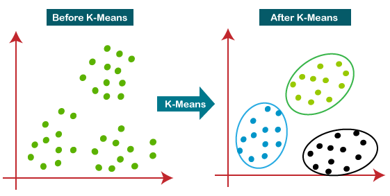
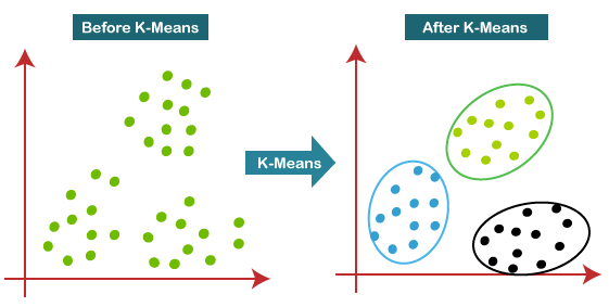
What is clustering?

To partition the observations into groups($clusters$) so that the pairwise dissimilarities between those assigned to the same cluster tend to be smaller than those in differenct clusters

Types of clustering algorithm

Type	Description	Example
Combinatorial algorithms	Work directly on the observed data with no direct reference to an underlyning probability model
Iterative descent clustering		K-means clustering
Mixture modeling	Supposes that the data is an i.i.d sample from some population described by a probability distribution function	Mixture model
Mode seekers	Take a nonparametric perspective, attempting to directly estimate distinct mode of the probability distribution function	Patient Rule Induction Method(PRIM), Generalized Association Rules
Hierachical clustering

Iterative greedy descent clustering

• An initial partition is specified
• At each iterative step, the cluster assignment are changed in such a way that the value of the criterion is improved from its previous value
• When the prescription is unable to provide an improvement, the algorithm terminates with the current assignmnet as its solution

---

Example data generation

• Make a toy data using make_blobs in sklearn!

from sklearn.datasets import make_blobs

x, y = make_blobs(n_samples=100, centers=3, n_features=2, random_state=7)
points = pd.DataFrame(x, y).reset_index(drop=True)
points.columns = ["x", "y"]
points.head()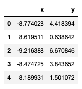

import seaborn as sns
sns.scatterplot(x="x", y="y", data=points, palette="Set2");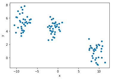

---

1. K-means

• The K-means algorithms is one of the most popular iterative descent clustering methods

Algorithm

	Given	Change
Step1	Cluster assignment	Change the means of cluster
Step2	A current set of means	Assigning of each observations

1. For a given cluster assignment, the total variance is minimized with respect to $\{m_{1},\dots,m_{K}\}$ yielding the means of the currently assigned cluster

2. Given a current set of means $\{m_{1},\dots,m_{K}\}$, the total variance is minimized by assigning each observation to the closest (current) cluster mean

3. Step 1 and 2 are iterated until the assignmnets do not change

Notice on intial centroids

• One should start the algorithm with many different random choices for the starting means, abd choose the solution having smallest value of the objective fucntion

---

2. Gaussian mixture

EM algorithm

Step	Given	Update
E step	Mixture component parameters	Responsibilities
M step	Responsibilities	Mixture component parameters

• E step
  • Assigns responsibilities for each data point based in its relative density under each mixture component
• M step
  • Recomputes the component density parameters based on the current responsibilities

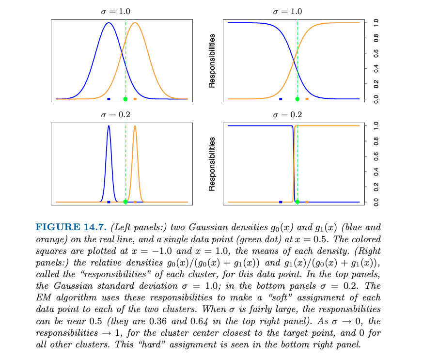
• Responsibilities
  • For given two density $g_0$ and $g_1$ and a data point $x$, the relative densities
    $\frac{g_0(x)}{g_0(x) + g_1(x)}, \quad\frac{g_1(x)}{g_0(x) + g_1(x)}$
    are called the $responsibility$ of each cluster, for this data point $x$

Gaussian mixture as soft K-means clustering

• EM algorithm is a soft version of K-means clustering, making probabilistic (rather than deterministic) assignments of points to cluster centers
• As $\sigma^2\to 0$, these probabilities become 0 and 1, and the two methods K-means and Gaussian mixture coincide

---

3. Hierachical clustering

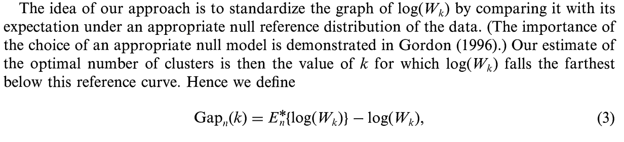
Gap statistics

Tibishirani proposed a statistic for choosing optimal number of clusters in 2001, called $gap\text{ }statistics$:

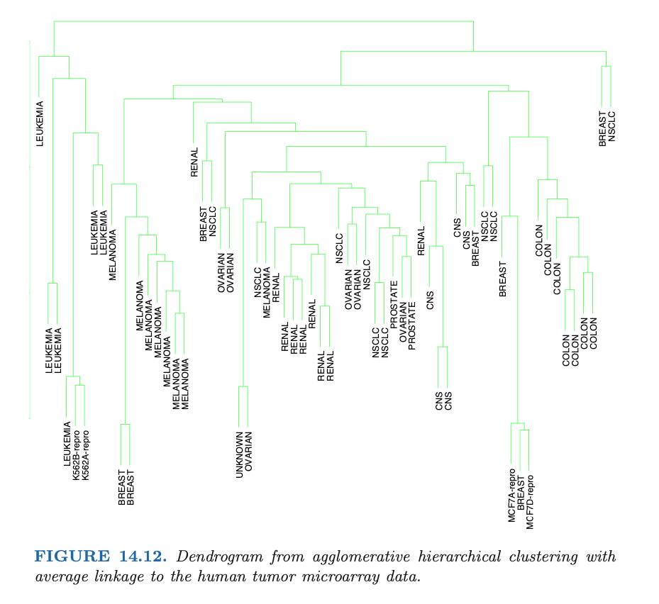
Dendrogram

A $dendrogram$ provides a highly interpretable complete description of the hierachical clustering in a graphical format.

Agglomerative vs. Divisive

Agglomerative	Divisive
Bottom up	Top down
Recursively merge	Recursively split
Begin with every observation representing a singleton cluster	Begin with the entire data set as a single cluster

• Agglomerative clustering
  • Begin with every observation representing a singleton cluster
  • At each of the $N-1$ steps, the closest two cluseters are merged into a single cluster, producing one less cluster at the next higher level
  • Therefore, a measure of dissimilarity between two clusters must be defined
• Divisive clustering
  • This approach has not been studied nearly as extensively as agglomerative methods in the clustering literature

Dissimilarity measures

Type	Formulation	Description
Single linkage	$d_{SL}(G,H)=\min\limits_{\substack{i\in G \\ i^{\prime}\in H}} d_{ii^{\prime}}$	- Violate the compactness property - i.e., produce clusters with very large diameters
Complete linkage	$d_{CL}(G,H)=\max\limits_{\substack{i\in G \\ i^{\prime}\in H}} d_{ii^{\prime}}$	- Violate the closeness property - i.e., observations assigned to a cluster can be much closer to members of the other clusters
Group average	$d_{GA}(G,H)=\frac{1}{N_G N_H}\sum\limits_{i\in G}\sum\limits_{i^{\prime}\in H}d_{ii^{\prime}}$	- Compromise SL and CL - But have invariance property
Ward linkage	$d_{W}(G,H)=ESS(GH)-[ESS(G)ESS(H)]$ where $ESS(X) = \sum\limits_{i=1}^{N_X} \lvert x_i - \frac{1}{N_X}\sum\limits_{i=j}^{N_X}x_j\rvert^2$ with

---

4. Self-Organizing Maps

What is Self-Organizing Maps(SOM)?

• The SOM procedure tries to bend the plane so that the buttons(green dots) approximate the data points as well as possible
  • The plane has the prototype(usually, centroid)
• Once the model is fit, the observations can be mapped down(projected) onto the two-dimensional grid

How to do SOM?

• By updating the prototypes! (green dots!)
• The observations $x_i$ are processed one at a time(these algorithms are called $online$). For each $x_i$,
  1. Fine the closest prototype $m_j$ to $x_i$ in Euclidean distance in $\mathbb{R}^{p}$
  2. For all neighbors $m_k$ of $m_j$, move $m_k$ toward $x_i$ via the update
     $m_{k} \gets m_{k} + \alpha(x_i - m_k)$
  • The neighbors of $m_j$ are defined to be all $m_k$ such that the distance between $\ell_{j}$ and $\ell_{k}$ is small
    • (NOTICE) That "distance" is defined in the integer topological coordinates of the prototypes, rather than in the feature space $\mathbb{R}^p$
  • The simplest approach uses Euclidean distance, and "small" is determined by a threshold $r$
  • The neighborhood of $m_j$ always includes $m_j$ itself
  • $\alpha$ is the learning rate
• In summary, SOM is
  • Input
    • data
    • Dimension of rectangular grid
  • Parameters
    • $\alpha$ : the learning rate
    • $r$ : the distance threshold
  • Output
    • Fitted prototypes
    • Projected retangular grid
• https://www.kaggle.com/code/izzettunc/introduction-to-time-series-clustering/notebook

SOM vs. K-means

---

5. Spectral clustering

Traditional clustering methods like $K$-means will not work well when the clusters are non-convex like below: (See Figure 14.29 in ESL p.546)

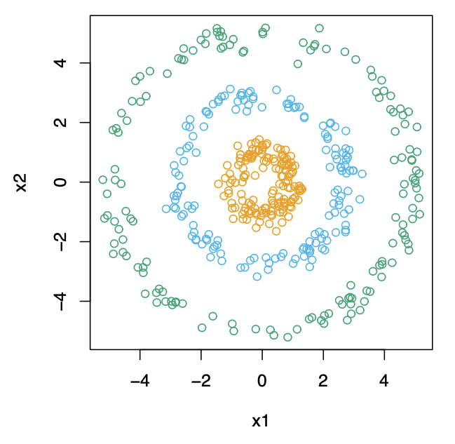
Spectral clustering is a generalization of standard clustering methods, and is designed for these situations

Clustering = graph-partition problem

Clustering can be rephrased as a graph-partition problem, with setup as below:

• a $N\times N$ matrix of pairwise similarities $s_{ii^{\prime}}\ge 0$ between all observation pairs
• represent the obeservations in an $undirected\text{ } similarity\text{ }graph$
  $G=<V,E>$
  • $V$ : the $N$ vertices $v_i$ representing the observations
  • $E$ : the edges connecting pairs of vertices if their similarity is positive, the edges are weighted by the $s_{ii^{\prime}}$

We wish to partition the graph, such that edges between different groups have low weight, and within a group have high weight. The idea of spectral clustering is to construct similarity graphs that represent the local neighborhood relationships between observations.

Graph Laplacian

The $graph\text{ }Laplacian$ is defined by

where

• $W$ : the matrix of edge weights $W=\{w_{ii^{\prime}}\}$ from a similarity graph is called the $adjacency\text{ }matrix$
• $G$ : a diagonal matrix with diagonal elements $g_i=\sum\limits_{i^{\prime}}w_{ii^{\prime}}$, the sum of the weights of the edges connected to it. This is called $degree\text{ }matrix$

Note that this is $unnormalized\text{ }graph\text{ }Laplacian$. There are a number of normalized versions have been proposed - for example, $\tilde{L}=I-G^{-1}W$.

Steps for spectral clustering

1. Define appropriate $similarity\text{ }graph$ (i.e., vertices and edges) that reflects local behavior of observations.

2. Get the $graph\text{ }Laplacian$ $L$ correspoding to the similarity graph $G$

3. Find the $m$ eigenvectors $Z_{N\times m}$ corresponding to the $m$ smallest eigenvalues of $L$ ($graph\text{ }Laplacian$, defined above). (For understanding, see this link and this link). This changes the data points from left to right. (See Figure 14.29 in ESL p.546)
   

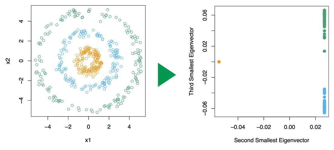
4. Using a standard method like $K$-means, cluster the rows of $Z$ to yield a clustering of the original data points

---

Performance evaluation

	Silhouette Coefficient	Calinski-Harabasz Index	Davies-Bouldin Index
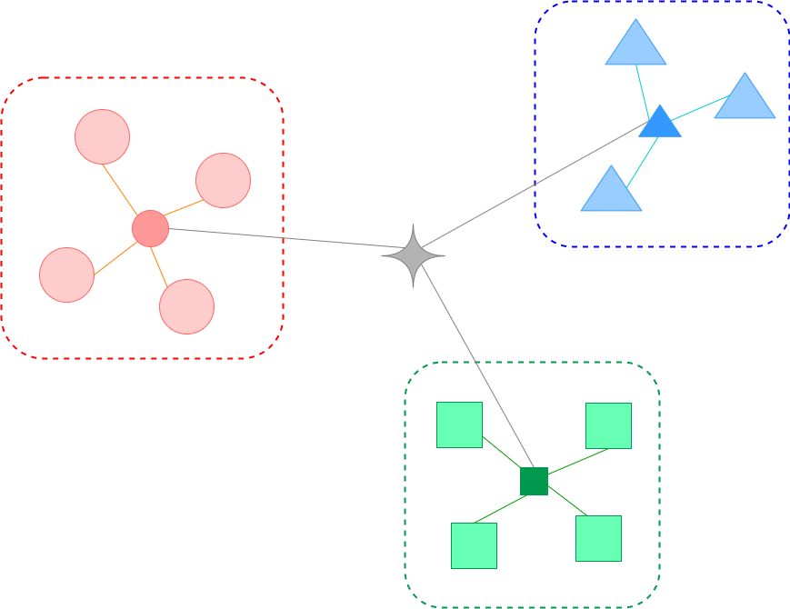	Mean of scaled differences between within-cluster distance and nearest-cluster distance	The ratio of the between-cluster dispersion and within-cluster dispersion	Mean of the average similarity between each cluster and its most similar(nearest) one
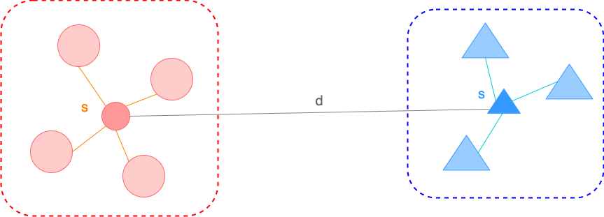
	For a single sample, $s=\dfrac{b-a}{\max(a, b)}$ where - $a$ : the mean distance between a sample and all other points in the same cluster - $b$ : the mean distance between a sample and all other points in the next nearest cluster For a set of samples, the mean of the Silhouette Coefficient for each sample	For a set of data $E$ of size $n_{E}$ which has been clustered into $k$ clusters, the Calinski-Harabasz score is defined as $s=\dfrac{tr(B_{k})}{tr(W_k)}\times\dfrac{n_{E}-k}{k-1}$ where - $tr(B_{k})$ : the trace of the between group dispersion matrix - $tr(W_{k})$ : the trace of the within-cluster dispersion matrix $W_{k}=\sum\limits_{q=1}^{K}\sum\limits_{x\in c_{q}}(x-c_{q})(x-c_{q})^{\top}$ $B_{k}=\sum\limits_{q=1}^{K}n_{q}(c_{q}-c_{E})(c_{q}-c_{E})^{\top}$ with - $C_{q}$ : the set of points in cluster $q$ - $c_q$ : the center of cluster $q$ - $c_{E}$ : the center of $E$	The Davies-Bouldin index is defined as $DB=\dfrac{1}{K}\sum\limits_{i=1}^{K}\max\limits_{i\ne j} R_{ij}$ where $R_{ij}=\dfrac{s_i + s_j}{d_{ij}}$ with - $s_i$ : the average distance between each point of cluster $i$ and the centroid of that cluster - $d_{ij}$ : the distance between cluster centroid $i$ and $j$

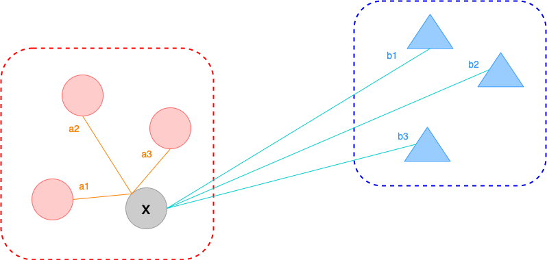
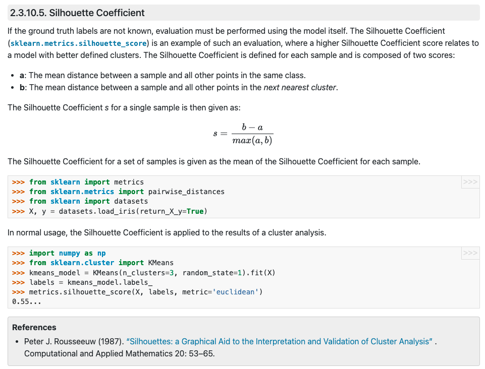
• Silhouette Coefficient
  • diff(within cluster distance, nearest cluster distance)
    • nearest cluster distance = min(between cluster distance)
  • For a given single sample point $x$,
    • within cluster distance $a = mean(a1,a2,...)$
    • nearest cluster distance $b = mean(b1,b2,...)$
      
  • (The Silhouette Coefficient for a set of samples)= mean(the Silhouette Coefficient for each sample)

• Calinski-Harabasz Index

  • (Between cluster variance)/(Within cluster variance)

  

• Davies-Bouldin Index

  • mean(nearest cluster similarity)

---

Choose optimal K

[References]

• Hastie, T., Tibshirani, R., Friedman, J. (2008) The Elements of Statistical Learning : Data Mining, Inference, and Prediction. Springer
• https://towardsdatascience.com/time-series-clustering-deriving-trends-and-archetypes-from-sequential-data-bb87783312b4
• https://scikit-learn.org/stable/modules/clustering.html#clustering-performance-evaluation