flights 데이터셋 활용해서 그래프 그리기
데이터 불러오기
import seaborn as sns
import matplotlib.pyplot as plt


flights_data = sns.load_dataset('flights')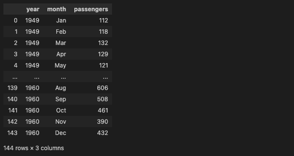
1. 연도 별 총 승객 수 with line graph
plt.figure(figsize=(10, 6))
plt.plot(flights_data.groupby('year')['passengers'].sum(), marker='o')
plt.title('Total Passengers per Year')
plt.xlabel('Year')
plt.ylabel('Total Passengers')
plt.grid(True)
plt.show()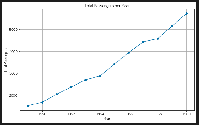
2. 연도 별 평균 승객 수 with bar graph
plt.figure(figsize=(10, 6))
plt.bar(flights_data['year'].unique(), flights_data.groupby('year')['passengers'].mean())
plt.title('Average Passengers per Year')
plt.xlabel('Year')
plt.ylabel('Average Passengers')
plt.show()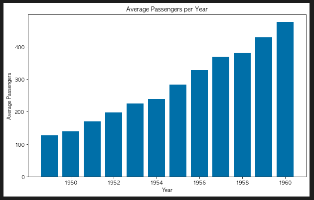
3. 승객 수 분포 with histogram
plt.figure(figsize = (10, 6))
plt.hist(flights_data['passengers'], bins = 20, edgecolor = 'black')
plt.title('Average Passengers per Year')
plt.xlabel('Year')
plt.ylabel('Average Passengers')
plt.show()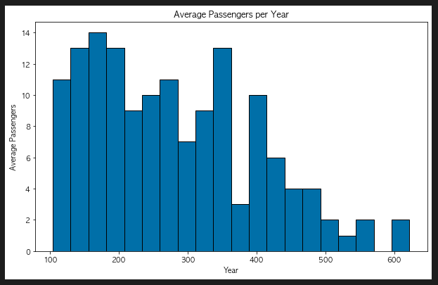
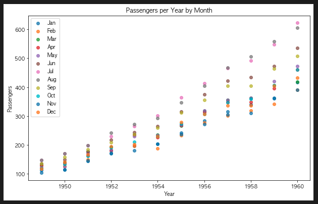
4. 연도 별 승객 수와 월간 승객 수 with scatter plot
plt.figure(figsize=(10, 6))
for month in flights_data['month'].unique():
    plt.scatter(flights_data[flights_data['month'] == month]['year'],
                flights_data[flights_data['month'] == month]['passengers'],
                label=month, alpha=0.7)
plt.title('Passengers per Year by Month')
plt.xlabel('Year')
plt.ylabel('Passengers')
plt.legend()
plt.show()
5. 월별 승객 수 분포
plt.figure(figsize=(8, 6))
plt.boxplot([flights_data[flights_data['month'] == month]['passengers'] for month in flights_data['month'].unique()],
            labels=flights_data['month'].unique())
plt.title('Passengers Distribution by Month')
plt.xlabel('Month')
plt.ylabel('Passengers')
plt.show()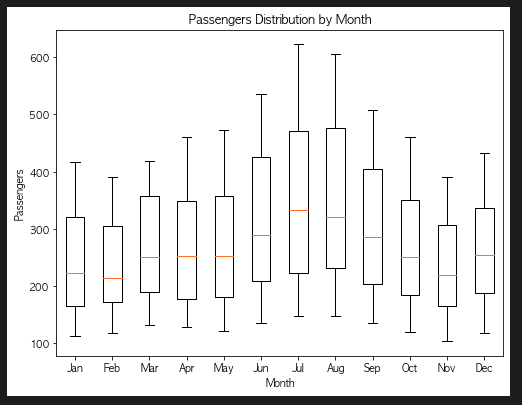
tips 데이터셋을 활용해서 그래프 그리기
1. 요일별 팁 금액 평균 with line chart
plt.figure(figsize=(8, 6))
tips_day = tips_data.groupby('day')['tip'].mean()
plt.plot(tips_day.index, tips_day.values, marker='o', linestyle='-', color='green')
plt.title('Average Tips by Day')
plt.xlabel('Day of the Week')
plt.ylabel('Average Tip Amount')
plt.grid(True)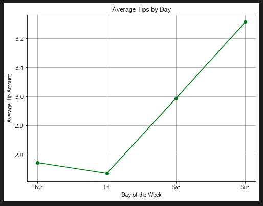
2. 요일별 총 팁 금액 with bar chart
plt.figure(figsize = (8, 6))
plt.bar(tips_data['day'].unique(),
        tips_data.groupby('day')['tip'].sum(),
        color = 'green')
plt.title('Total Tips by Day')
plt.xlabel('Day of the Week')
plt.ylabel('Total Tip Amount')
plt.show()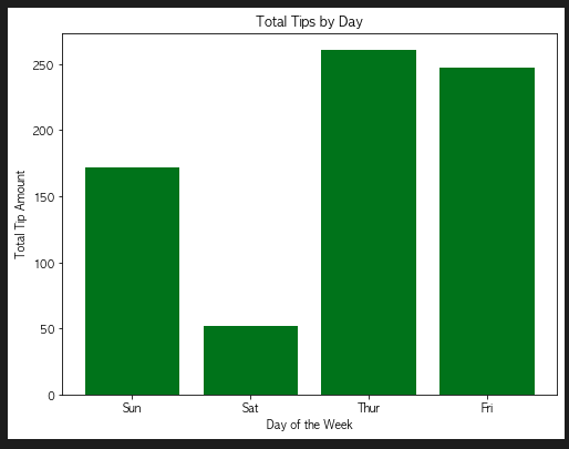
3. 식사 금액 분포 with histogram
plt.figure(figsize = (8, 6))
plt.hist(tips_data['total_bill'], bins = 20,
         color = 'skyblue', edgecolor = 'black', alpha = 0.7)
plt.title('Distribution of Total Bill')
plt.xlabel('Total Bill Amount')
plt.ylabel('Frequency')
plt.show()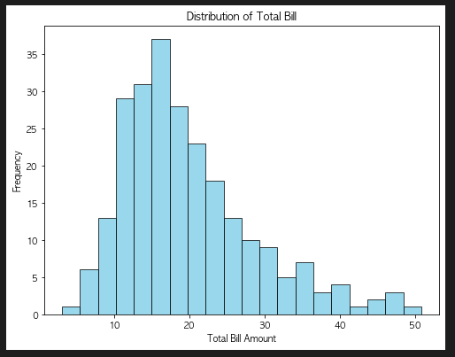
4. 식사 금액과 팁 금액의 관계 with scatter plot
plt.figure(figsize = (8, 6))
plt.scatter(tips_data['total_bill'], tips_data['tip'], alpha = 0.7)
plt.title('Tip Amount vs Total Bill')
plt.xlabel('Total Bill Amount')
plt.ylabel('Tip Amount')
plt.show()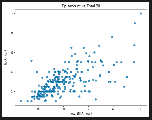
5. 요일별 식사 금액 분포 with box plot
matplotlib으로 그리기
plt.figure(figsize = (8, 6))
plt.boxplot([tips_data[tips_data['day'] == day]['total_bill'] for day in tips_data['day'].unique()],
             labels = tips_data['day'].unique())
plt.title('Total Bill Distribution by Day')
plt.xlabel('Day of the Week')
plt.ylabel('Total Bill Amount')
plt.show()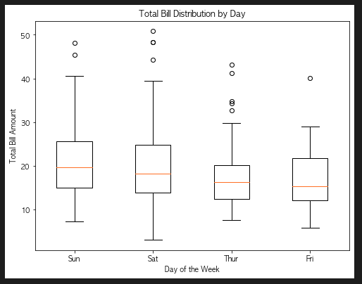
seaborn으로 그리기
plt.figure(figsize = (8, 6))
sns.boxplot(x = 'day', y = 'total_bill', data = tips_data)
plt.title('Total Bill Distribution by Day')
plt.xlabel('Day of the Week')
plt.ylabel('Total Bill Amount')
plt.show()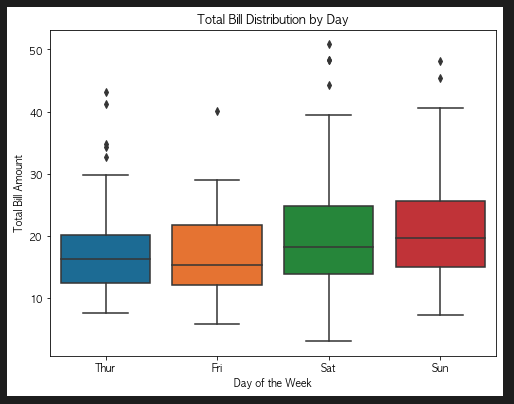

To Dare is To Do