1. Introduction
가중치 그래프는 기존의 그래프에 weight, 즉 정점간 거리가 추가된 그래프이다. 이 글에선 최소 비용 신장트리와 최단경로, 위상 순서를 알아보도록 하겠다.
2. Contents
2.1. 최소 비용 신장트리
최소 비용 신장 트리는 트리를 구성하는 간선들의 가중치를 합한 것이 최소가 되는 신장트리이다. 최소 비용 신장트리를 구하는 알고리즘들 중 Kruskal, Prim 알고리즘에 대해 알아보도록 하자.
최소 비용 신장트리를 구현하기 위해 간선을 표현하기 위한 Edge 클래스, 비용이 작은 간선을 선택하는 MinHeap 과 연결여부를 판단하는 UnionFind를 사용한다.
interface CompKey {
    public int compareTo(Object o);
}
class Edge implements CompKey {
int head;
int tail;
int weight;
public Edge(int h, int t, int w) {
head = h;
tail = t;
weight = w;
}
public int compareTo(Object value) {
int a = this.weight;
int b = ((Edge)value).weight;
return a - b;
}
}class MinHeap {
private int count;
private int size;
private CompKey[] itemArray;
public MinHeap() {
count = 0;
size = 64;
itemArray = new CompKey[size];
}
public MinHeap(CompKey[] origArray) {
count = origArray.length - 1;
size = count + 1;
itemArray = origArray;
int childLoc;
int currentLoc;
for (currentLoc=count/2; currentLoc > 0; currentLoc--) {
childLoc = currentLoc*2;
while (childLoc <= count) {
if (childLoc < count) {
if (itemArray[childLoc+1].compareTo(itemArray[childLoc]) < 0)
childLoc++;
}
if (itemArray[currentLoc].compareTo(itemArray[childLoc]) <= 0) break; // ??
else {
CompKey temp = itemArray[currentLoc];
itemArray[currentLoc] = itemArray[childLoc];
itemArray[childLoc] = temp;
currentLoc = childLoc;
childLoc = currentLoc * 2;
} // else
} // while
} // for
}
public void insert(CompKey newItem) {
if (count >= size -1) {
System.out.println();
return;
}
count++;
int childLoc = count;
int parentLoc = childLoc / 2;
while (parentLoc != 0) {
if (newItem.compareTo(itemArray[parentLoc]) >= 0) {
itemArray[childLoc] = newItem;
return;
} else {
itemArray[childLoc] = itemArray[parentLoc];
childLoc = parentLoc;
parentLoc = childLoc / 2;
}
}
itemArray[childLoc] = newItem;
}
public CompKey delete() {
if (count == 0) {
return null;
} else {
int currentLoc;
int childLoc;
CompKey itemToMove;
CompKey deletedItem;
deletedItem = itemArray[1];
itemToMove = itemArray[count--];
currentLoc = 1;
childLoc = 2*currentLoc;
while (childLoc <= count) {
if (childLoc < count) {
if (itemArray[childLoc+1].compareTo(itemArray[childLoc]) < 0)
childLoc++;
}
if (itemArray[childLoc].compareTo(itemToMove) < 0) {
itemArray[currentLoc] = itemArray[childLoc];
currentLoc = childLoc;
childLoc = 2*currentLoc;
} else {
itemArray[currentLoc] = itemToMove;
return deletedItem;
}
} // while
itemArray[currentLoc] = itemToMove;
return deletedItem;
} //else
}
public int numberElements() {
return count;
}
}class UnionFind {
int [] parent;
public UnionFind(int n) {
parent = new int[n];
for (int i = 0; i < n; i++)
parent[i] = i;
}
private int root(int i) {
while (i != parent[i]) {
parent[i] = parent[parent[i]];
i = parent[i];
}
return i;
}
public boolean find(int p, int q) {
return root(p) == root(q);
}
public void union(int p, int q) {
int i = root(p);
int j = root(q);
parent[i] = j;
}
}2.1.1 Kruskal Algorithm
크루스칼 알고리즘은 한번에 하나의 간선을 선택, 최소 비용 신장트리에 추가하는 방법이다. 그래프에서 비용이 가장 작은 간선을 선정하되, 이미 추가한 간선들과 사이클을 형성하지 않는 선에서만 추가한다.
이제 kruskal 메소드를 구현해보자.
	public Edge[] kruskal() {
		Edge[] T = new Edge[n-1]; // 선택한 간선
		int Tptr = -1;

		MinHeap edgeList = new MinHeap(); // 그래프의 모든 간선을 추가

		for(int i=0;i<n;i++) {
			for(int j=0;j<i;j++) {
				if(weight[j][i] == 9999 || weight[j][i] == 0) continue; // 위 그래프에선 연결되지 않은 간선간 거리를 9999로 설정해놓았다.
				edgeList.insert(new Edge(j, i, weight[j][i]));
			}
		}

		UnionFind uf = new UnionFind(n);

		while(edgeList.numberElements() != 0) {
			Edge tmp = (Edge)edgeList.delete();
			if(!uf.find(tmp.head, tmp.tail)) { // 연결여부 판별
				uf.union(tmp.head, tmp.tail); // Union에 추가
				T[++Tptr] = tmp; // 사이클이 없는 간선을 추가
			}
		}
		return T;
	}
2.1.2 Prim Algorithm
프림은 한번에 하나의 간선을 선택하여 T에 추가한다. 이 때 크루스칼 알고리즘과 다른 점은 전 과정을 하나의 트리만을 유지하며 확장한다는 것이다.
이제 프림 알고리즘을 구현해보자.
	public Edge[] prim(int i) {
		Edge[] T = new Edge[n-1];
		int Tptr = -1;
		MinHeap edgeList = new MinHeap();

		for(int j=0;j<n;j++) {
			if(weight[i][j] == 0 || weight[i][j] == 9999) continue;
			edgeList.insert(new Edge(i, j, weight[i][j])); // 시작 정점에 연결된 간선을 추가
		}

		UnionFind uf = new UnionFind(n);

		while(Tptr < n-2) {
			Edge tmp = (Edge)edgeList.delete();
			if(!uf.find(tmp.head, tmp.tail)) {
				uf.union(tmp.head, tmp.tail); // 사이클이 아니라면 추가
			 	T[++Tptr] = tmp; // 최소간선리스트에 추가
				for(int k=0;k<n;k++) { // 현재 추가한 간선과 연결된 간선을 전부 추가
					if(weight[tmp.tail][k] == 0 || weight[tmp.tail][k] == 9999) continue;
					edgeList.insert(new Edge(tmp.tail, k, weight[tmp.tail][k]));
				}
			}
		}
		return T;
	}
2.2. 최단 경로
최단경로는 크게 2가지로 구분하는데, 음의 가중치가 있는지 없는지에 따라 나눠진다.
음의 가중치가 없다면 다익스트라, 있다면 벨만&포드 알고리즘으로 최단 경로를 구한다.
2.2.1 Dijkstra Algorithm
다익스트라는 첫 정점을 추가하고 그 정점에서 가장 작은 가중치를 가진 간선을 선택한다. 그 후 선택된 간선을 경유해 가는 가중치를 계산해 더 작다면 갱신해준다.
	public int[] shortestPath(int v) {
		boolean s[] = new boolean[n]; // 최단거리가 정해졌는지 파악
		int dist[] = new int[n]; // 최단거리 간선 리스트
		int u;

		for (int i = 0; i < n; i++) {
			dist[i] = weight[v][i]; // 선택된 간선에서 시작하는 가중치
		}

		s[v] = true; // 현재 정점 방문상태로 변경
		dist[v] = 0; // 현재 가중치 0으로 설정

		for (int i = 0; i < n - 2; i++) {
			int min_dist = 9999;
			u = 0;

			for (int j = 0; j < n; j++) { // 가중치가 가장 작은 간선 선택
				if (s[j])
					continue;
				if (dist[j] < min_dist) {
					min_dist = dist[j];
					u = j; // 인덱스를 저장해놨다가
				}
			}

			dist[u] = min_dist; // 갱신
			s[u] = true; // 방문 설정

			for (int w = 0; w < n; w++) {
				if (!s[w]) { // 방문하지 않은 간선 중
					if (dist[w] > dist[u] + weight[u][w]) // 최단거리를 경로해서 가는게 더 짧다면 갱신
						dist[w] = dist[u] + weight[u][w];
				}
			}
		}
		return dist;
	}
2.2.2 Bellman and Ford Algorithm
음의 가중치가 존재하는 그래프의 최단 경로를 파악하는 건 다익스트라 알고리즘으로 불가능하다. 음의 사이클이 존재한다면 최단경로가 무한대로 갱신되기 때문이다.
이 때문에 벨만&포드 알고리즘은 사이클이 없는 최단 경로가 가질 수 있는 최대 간선 수를 이용한다.
만약 최대 간선수보다 더 갱신을 시도했을 때 가중치가 갱신된다면 음의 가중치가 존재함을 알 수 있다.
public int[] negativePath(int v) {
int dist[] = new int[n];
for (int i = 0; i < n; i++) {
dist[i] = weight[v][i];
}
dist[v] = 0;
for (int i = 0; i < n - 2; i++) { // n-2번 시행
for (int j = 0; j < n; j++) {
if (dist[j] != 9999 || dist[j] != 0) {
for (int k = 0; k < n; k++) {
if (dist[k] > dist[j] + weight[j][k]) {
dist[k] = dist[j] + weight[j][k];
}
}
}
}
}
return dist;
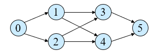
}2.3. 위상 경로
위상 정렬은 선행자가 존재하는 그래프일 때 선행자가 반드시 먼저 나와야하는 경로이다.
위상 정렬의 경우 Graph의 멤버에 선행자의 수를 저장하는 indegree, 선행자가 없는 큐인 zeroPredQ, 정렬된 리스트인 sortedList와 후행자를 담고있는 큐가 필요하다. 여기선 Node의 배열로 Queue를 대신하였다.
    public Graph(int noOfVertices) {
    	n = noOfVertices;
//    	Q = new Queue[n];
    	header = new Node[n];
    	zeroPredQ = new Queue();
    	sortedList = new int[n];
//    	for(int i=0;i<n;i++) {
//    		Q[i] = new Queue();
//    	}
    	indegree = new int[n];
    }
선행자에 대한 처리를 해주어야 하기 때문에 insert 메소드도 변경이 필요하다.
    public void insertEdge(int i, int j) {
    	Node node1 = new Node();
    	node1.vertex = j;
    	node1.link = header[i];

    	header[i] = node1;

    	indegree[j]++;
    }
위상정렬 메소드는 다음과 같다.
    public void topologicalSort() {
    	int i, v, successor;
    	for(i=0;i<n;i++) {
    		if(indegree[i]==0) { // 선행자가 없는 정점을 zeroPredQ에 추가
    			zeroPredQ.enqueue(i);
    		}
    	}
    	if(zeroPredQ.isEmpty()) { // 선행자가 없는 정점이 존재하지 않으면
    		System.out.println("network has a cycle"); // 사이클이 존재하는 것임
    		return;
    	}

    	int count = 0;
    	while(!zeroPredQ.isEmpty()) {
    		v = zeroPredQ.dequeue(); // 값을 꺼내
    		sortedList[count++] = v; // 정렬된 리스트에 추가

    		if(header[v] == null) continue;
    		else {
    			successor = header[v].vertex; // successor를 후행자로 갱신
    			header[v] = header[v].link;
    		}
    		while(true) {
    			indegree[successor]--; // 진입차수 감소
    			if(indegree[successor] == 0)  zeroPredQ.enqueue(successor); // 감소된 진입차수가 0이 된다면 zeroPredQ에 추가
    			if(header[v] != null) {
        			successor = header[v].vertex; //successor 갱신
        			header[v] = header[v].link;
    			}
    			else break;
    		}
    	}
    	System.out.println("Topological Order is : ");

    	for(int k=0;k<sortedList.length;k++) {
    		System.out.print(sortedList[k] + " ");
    	}
    }
4. Review
가중치 그래프에서의 최소 비용 신장 트리와 최단 경로, 위상 순서에 대해 알아보았다. 이전에 하던 내용에 비해 알고리즘이 복잡해지고 생각할 것이 많아져서인지 학습하는데 더 재밌는 부분이였다.
시험기간동안 내용을 기록할 시간이 없어서 약 3주간 공백이 생겨버렸다.. 시험도 끝났으니 모아놨던 정리할 내용들을 얼른 정리하고 새로운 내용을 공부해야겠다!
다음은 정렬기법 중 선택정렬, 버블정렬, 삽입정렬, 그리고 힙정렬에 대해 알아보겠다!