Classification
불연속(discrete), 분류 문제
Examples
- Spam / Not Spam
- Yes / No
c.f) Regression: 연속된 실수 예측
분류 문제를 regression으로 해결한다면
- Threshold hθ(x) at 0.5
- if hθ(x)≥0.5, predict y=1
- error - 예측값과의 오차로 계산한다면 학습이 제대로 되지 않는다.
- 출력값의 범위가 0, 1을 벗어난다. - 모든 실수
- Classificaiton: y=0 or y=1
- hθ(x)는 1 초과, 0 미만일 수 있다.
- Logistic Regression: 0≤hθ(x)≤1
Hypothesis Representation
Logistic Regression Model
이름이 회귀이지만 분류 문제를 해결하기 위한 모델이다.
Goal: 0≤hθ(x)≤1
선형 회귀 hypothesis: hθ(x)=θTx
→ Classification hypothesis
- 0 이상 1 이하의 실수여야 한다.
- Sigmoid function(logistic function)을 이용해서 출력 범위를 0 이상 1 이하로 제한한다. - regression과 유사
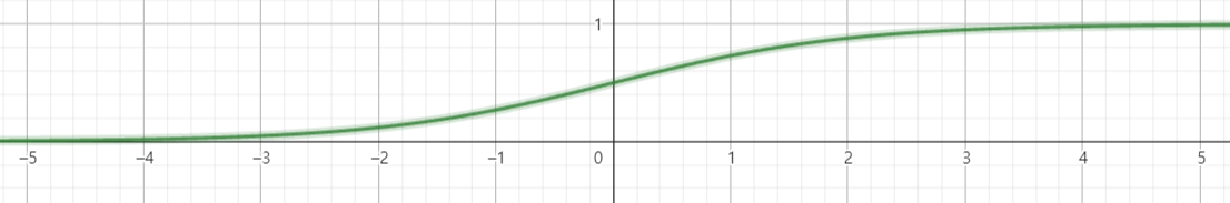
- sigmoid function은 확률 모델로 바꾸어주는 역할
- 0.5를 기준으로 최종 output을 0 또는 1로 설정한다.
hθ(x)=g(θTx)
g(z)=1+e−z1,z=θTx
- x에 따라 z가 적절히 분배되도록 θ가 학습된다.
Interpretation of Hypothesis Output
input x에 대한 출력 hθ(x)를 y=1이 되게 하는 probability로 간주한다.
- 암 세포에 대한 양성 예측 hθ(x)=0.7,y=1
- hθ(x)=P(y=1∣x;θ)
- y=0 or y=1
- P(y=0∣x;θ)+P(y=1∣x;θ)=1
Decision boundary
경계선(boundary)을 기준으로 값을 결정한다.
- Sigmoid Function
- predict y=1 if hθ(x)≥0.5,θTx≥0
- predict y=0 if hθ(x)<0.5,θTx<0
Cost Function
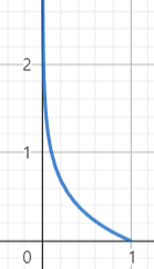
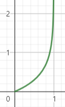
Cost(hθ(x),y)={−log(hθ(x))−log(1−hθ(x))if y=1if y=0
- 1이 정답이라면 1에 가까울수록 0으로 수렴한다.
- Cost(hθ(x),y)=−ylog(hθ(x))−(1−y)log(1−hθ(x))
Simplified cost function and gradient descent
- J(θ)=−m1∑i=1m[y(i)loghθ(x(i))+(1−y(i))log(1−hθ(x(i)))]
θ에 대한 미분
f=loghθ(x),t=hθ(x)
∂θj∂f =∂t∂f∂θj∂t =tln101∂θ∂t =ln101+e−θTx∂θj∂t
∂θj∂t= ∂θTx∂t∂θj∂θTx= (1+e−θTx1)(1−1+e−θTx1)∂θj∂θTx
∂θj∂θTx= xj
(1−1+e−θTx1)xj
Multi-class classification: One-vs-all
Multiclass classification
class가 세 가지 이상인 경우 각 class에 대해 모델을 사용한다.
- 특정 데이터가 입력되었을 때
- class 1 40%
- class 2 20%
- class 3 20%
와 같이 확률의 합이 1이 아닐 수 있다.
P(y=i∣x;θ),(i=1,2,3)
- 새로운 입력 x에 대해 maxihθ(i)(x)를 출력으로 예측한다.