pandas[2]

Hyunwoo Lee·2022년 3월 28일

Selection and drop

selection

데이터를 가져오는 것

df['ten']

0       2.31
1       7.07
2       7.07
3       2.18
4       2.18
       ...

column을 list 형태로 주면 1개 이상의 특정 column을 선택할 수도 있다.

df[["six", "nine", 'seven']]

	six	nine	seven
0	18.0	0.00632	24.0
1	0.0	0.02731	21.6
2	0.0	0.02729	34.7
3	0.0	0.03237	33.4
4	0.0	0.06905	36.2
...	...	...	..

df[["six"]]

	six
0	18.0
1	0.0
2	0.0
3	0.0
4	0.0
...	...

2차원 배열을 넣어주면 data frame으로, 1차원 배열을 넣으면 series로 출력된다.

df[0:4]

	nine	six	ten	twelve	eleven	eight	five	ZN	four	CRIM	INDUS	three	thirteen	seven
0	0.00632	18.0	2.31	0	0.538	6.575	65.2	4.0900	1	296.0	15.3	396.90	4.98	24.0
1	0.02731	0.0	7.07	0	0.469	6.421	78.9	4.9671	2	242.0	17.8	396.90	9.14	21.6
2	0.02729	0.0	7.07	0	0.469	7.185	61.1	4.9671	2	242.0	17.8	392.83	4.03	34.7
3	0.03237	0.0	2.18	0	0.458	6.998	45.8	6.0622	3	222.0	18.7	394.63	2.94	33.4

숫자를 넣어주면 row index에 해당하는 값만 불러온다.

df[0:4][["nine", 'six']]

	nine	six
0	0.00632	18.0
1	0.02731	0.0
2	0.02729	0.0
3	0.03237	0.0

row index와 column이름을 같이 사용하면 이렇게 불러올 수도 있다.

boolean selection

df[df['six'] >0]

	nine	six	ten	twelve	eleven	eight	five	ZN	four	CRIM	INDUS	three	thirteen	seven
0	0.00632	18.0	2.31	0	0.538	6.575	65.2	4.0900	1	296.0	15.3	396.90	4.98	24.0
6	0.08829	12.5	7.87	0	0.524	6.012	66.6	5.5605	5	311.0	15.2	395.60	12.43	22.9
7	0.14455	12.5	7.87	0	0.524	6.172	96.1	5.9505	5	311.0	15.2	396.90	19.15	27.1
8	0.21124	12.5	7.87	0	0.524	5.631	100.0	6.0821	5	311.0	15.2	386.63	29.93	16.5
9	0.17004	12.5	7.87	0	0.524	6.004	85.9	6.5921	5	311.0	15.2	386.71	17.10	18.9

True인 index만 selection할 수도 있다.

s_data[list(range(0, 10, 3))]

0    0.00632
3    0.03237
6    0.08829
9    0.17004
Name: nine, dtype: float64

list 형태도 가능

iloc, loc

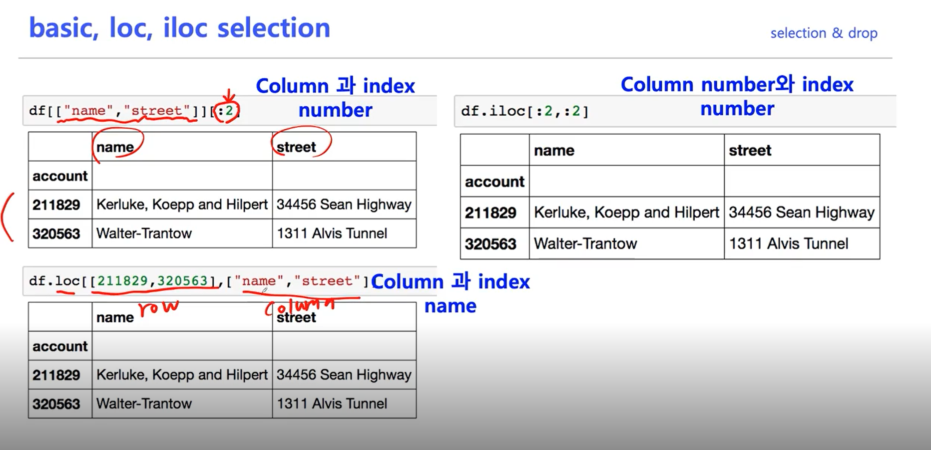
indexing

df3.index = list(range(5, 8, 1))

nine	six	ten	twelve	eleven	eight	five	ZN	four	CRIM	INDUS	three	thirteen	seven
5	0.00632	18.0	2.31	0	0.538	6.575	65.2	4.0900	1	296.0	15.3	396.90	4.98	24.0
6	0.02731	0.0	7.07	0	0.469	6.421	78.9	4.9671	2	242.0	17.8	396.90	9.14	21.6
7	0.02729	0.0	7.07	0	0.469	7.185	61.1	4.9671	2	242.0	17.8	392.83	4.03	34.7

이렇게 인덱싱을 바꿀 수도 있다.

df_r = df3.reset_index()
df_r

	index	nine	six	ten	twelve	eleven	eight	five	ZN	four	CRIM	INDUS	three	thirteen	seven
0	5	0.00632	18.0	2.31	0	0.538	6.575	65.2	4.0900	1	296.0	15.3	396.90	4.98	24.0
1	6	0.02731	0.0	7.07	0	0.469	6.421	78.9	4.9671	2	242.0	17.8	396.90	9.14	21.6
2	7	0.02729	0.0	7.07	0	0.469	7.185	61.1	4.9671	2	242.0	17.8	392.83	4.03	34.7

reset index를 하면 index가 추가로 생성된다.

drop=True로 하면 기존 index는 사라진다
inplace=True를 하면 실제로 df의 값이 바뀐다(할당 필요 없음)

Drop

df.drop(1)

1번 index가 삭제된다.
axis를 넣어 column이나 row를 선택하여 삭제할 수 있다.

small_df.drop('nine', axis=1)

	six	ten
0	18.0	2.31
1	0.0	7.07
2	0.0	7.07
3	0.0	2.18

마찬가지로 implace=True를 하면 자기 자신에서 삭제할 수 있다.

dataframe operations

s1 = Series(data=range(1,5), index=list("abcd"))
s2 = Series(data=range(5,11), index=list("bcdefg"))

s1 + s2

a     NaN
b     7.0
c     9.0
d    11.0
e     NaN
f     NaN
g     NaN
dtype: float64

index가 겹치는경우 연산수행, 없으면 NaN

dataframe도 마찬가지이다.

df1 = pd.DataFrame(data = np.arange(9).reshape(3, 3), columns=list('abc'))

	a	b	c
0	0	1	2
1	3	4	5
2	6	7	8

df2 = pd.DataFrame(data=np.arange(16).reshape(4,4), columns=list('abcd'))

a	b	c	d
0	0	1	2	3
1	4	5	6	7
2	8	9	10	11
3	12	13	14	15

df1 + df2

	a	b	c	d
0	0.0	2.0	4.0	NaN
1	7.0	9.0	11.0	NaN
2	14.0	16.0	18.0	NaN
3	NaN	NaN	NaN	NaN

df1.add(df2, fill_value=0)를 쓰면 자동으로 NaN대신 0을 채워준다.

series + dataframe

df1.add(s1, axis=0)
	a	b	c
0	0	1	2
1	4	5	6
2	8	9	10

axis를 정해주면 broadcasting되어 실행된다.

lambda & map

lambda

f = lambda x : x**2
f(df1)

a	b	c
0	0	1	4
1	9	16	25
2	36	49	64

map

변환하는 함수

list(map(lambda x: x+5, df))
[5, 6, 7, 8, 9, 10, 11, 12, 13, 14, 15, 16, 17, 18]

z = {1:'a', 2:'b', 3:'c'}
s1.map(z)

0    NaN
1      a
2      b
dtype: object

def f (x):
    if x >0:
        return 1
    else:
        return 0

df.iloc[:][1].map(f)  
0      1
1      0
2      0
3      0
4      0
      ..

df[1].unique() 실행시 중복되는 값을 제거하고 한 번씩만 보여준다.

apply

map과 달리 Series 전체(column)에 대한 함수를 적용
입력 값이 시리즈 데이터로 입력받아 handling가능

f = lambda x : x.max() - x.min()
df.apply(f)

0      88.96988
1     100.00000
2      27.28000
3       1.00000
4       0.48600
5       5.21900
6      97.10000
7      10.99690
8      23.00000
9     524.00000
10      9.40000
11    396.58000
12     36.24000
13     45.00000
dtype: float64

df.apply(np.mean)

0       3.613524
1      11.363636
2      11.136779
3       0.069170
4       0.554695
5       6.284634
6      68.574901
7       3.795043
8       9.549407
9     408.237154
10     18.455534
11    356.674032
12     12.653063
13     22.532806
dtype: float64