Prologue

많은 교재와 강의에서 back prop을 정리할 때 node차원에서만 바라보는 게 아쉬웠다. 그러면 scratch로 신경망을 구현할 때 back prop에서 막히고 만다. 나는 동적인 신경망을 만들고 싶었다. 그래서 조금은 더 깊게 파봤다.

Basic archetecture

인공신경망은 입력값을 받아서 1. weight($W$)와 곱한 다음(bias는 생략하기로 한다.) 2. 활성화함수($\sigma$, 시그모이드 함수)로 결과값을 내보낸다.

$f=x\cdot W$
$z=\sigma(f)$

이 두 함수가 하나의 레이어를 구성하는데 이전 레이어의 결과값은 다음 레이어의 입력값이 되는 방식으로 여러겹 쌓아서 신경망을 만든다. 우리가 할 일은 결과값을 실제값과 최대한 같게 하는 가중치들을 찾는 것이다. 가중치를 여기저기 마구 찍어보면서 찾아도 되지만 이렇게 최적값을 찾는 건 귀막고 눈감은 채 친구찾는 기분일 거다. 이것보다 좀더 과학적으로 접근해보자고 제시한 방법이 back propagation과 gradient descent다. 이 때 핵심이 연쇄법칙이다.

All we need is Chain rule

위의 예시에서 우리는 $z$함수의 $W$에 대한 변화량을 알고 싶지만 직접적으로 연관이 있지는 않다. 그럴 때 쓰라고 머리 좋은 사람들이 만들어 놓은 게 chain rule이다.

${\partial z\over \partial W}={\partial z\over \partial f}{\partial f\over\partial W}$

이 점을 숙지하고 따라가면 좀 수월할 거라 생각한다.

Calculating gradient

3 레이어 네트워크에서 가중치를 업데이트하는데 필요한 변화량을 생각해보기 전에 신경망을 시각적으로 풀어보면 아래와 같이 생겼다.

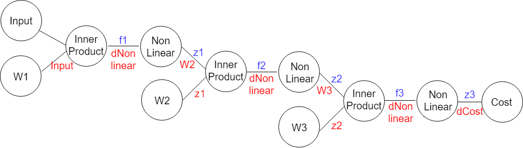
이렇게 해놓으면 복잡한 합성함수 속에서도 원하는 변화량을 잘 포착할 수 있다. 앞서 서술했듯이 우리는 각 가중치들이 변할 때 비용함수가 얼마나 변하는지 찾을 거다. 이런 관점에서 필요한 것은 ${\partial C\over \partial W_1}\ \ {\partial C\over \partial W_2},\ \ {\partial C\over \partial W_3}$ 이렇게 세 가지가 되겠다. 그래프를 따라가면서 손실함수의 각 가중치에 대한 변화량은 아래와 같이 정리할 수 있다.

${\partial C \over \partial W_3}={\partial C \over \partial z_3}{\partial z_3 \over \partial f_3}{\partial f_3 \over \partial W_3}= \partial \text{Cost} \cdot \partial \sigma(f3) \cdot z_2$

${\partial C \over \partial W_2}={\partial C \over \partial z_3}{\partial z_3 \over \partial f_3}{\partial f_3 \over \partial z_2}{\partial z_2 \over \partial f_2}{\partial f_2 \over \partial W2}= \partial \text{Cost} \cdot \partial \sigma(f3) \cdot W_3 \cdot \partial \sigma(f2) \cdot z_1$

${\partial C \over \partial W_1} = {\partial C \over \partial z_3}{\partial z_3 \over \partial f_3}{\partial f_3 \over \partial z_2}{\partial z_2 \over \partial f_2}{\partial f_2 \over \partial z_1}{\partial z_1 \over \partial f_1}{\partial f_1 \over \partial W1}= \partial \text{Cost} \cdot \partial \sigma(f3) \cdot W_3 \cdot \partial \sigma(f2)\cdot W_2\cdot\partial \sigma(f1)\cdot \text{Input}$

물론 이 순서대로 행렬을 곱했다가는 연산이 안 되는 문제에 부닥친다. 그래서 각 레이어에서 local gradient를 구할 때 이런 패턴으로 계산한다.

$\partial C = C'(z_n)\odot \sigma'(f_n)$
$\delta_n = w_{n+1}^T\cdot\delta_{n+1}\odot \sigma'(f_n)$

여기에서 $\cdot,\ \ \odot$요 두 연산은 모두 행렬곱이고 각각 inner(dot) product, hadamard product라고 부른다. 이제 이 과제에서 활성화 함수를 시그모이드로 정하고 패턴대로 정리하면 이렇게 된다.

${\partial C \over \partial W_3}=2(f_3-Gt)\cdot z_2^T$
${\partial C \over \partial W_2}= {W_3}^T\cdot2(f_3-Gt)\odot \sigma(f2)(1-\sigma(f2))\cdot z_1^T$
${\partial C \over \partial W_1}= {W_2}^T\cdot \{{W_3}^T\cdot2(f_3-Gt)\odot \sigma(f2)(1-\sigma(f2)\}\odot \sigma(f1)(1-\sigma(f1))\cdot x^T$

이쯤 되면 각 레이어의 그래디언트를 연산하는 규칙이 보인다.

$\text{Gradient}=\text{local gradient}\times \text{output of prior layer}$

Put these all together

import matplotlib.pyplot as plt
import numpy as np

def layer(X: np.array, units: int, activation: str = None):
    """
    X: input matrices of each layer and it decides weight matrix shape.
    units: decides number of nodes in a hidden layer
    activation: decides weight initialization. He, Xaiver and LeCun initialization are available.
    """
    h, w = X.shape
    if activation == 'relu':
        weight = np.random.randn(w, units) * np.sqrt(2 / w)  # He initialization
    elif activation == 'tanh' or activation == 'softmax':
        weight = np.random.randn(w, units) * np.sqrt(1 / w)  # Xavier initialization
    elif activation is None:
        weight = np.random.randn(w, units) * 0.01  # LeCun initialization
    return weight

def relu(X, props: str = 'fwd'):
    """
    X: input matrices.
    props: decides propagate direction e.g. fwd means forward pass and bwd means backward pass.
    """
    if props == 'fwd':
        return np.maximum(0, X)
    elif props == 'bwd':
        return np.greater(0, X).astype(int)
    
def softmax(X):
    """
    X: input matrices.
    I didn't create derivitives of softmax because when back propagation it's much efficient 
    to calculate it with cross entropy
    """
    score = np.exp(X)
    return score / np.sum(score, axis = 1, keepdims = True)

def cross_entropy(X, Y, props: str = 'fwd'):
    """
    X: input matrices
    Y: label vector
    props: decides propagate direction e.g. fwd means forward pass and bwd means backward pass.
    """
    n = len(X)
    if props == 'fwd':
        likelyhood = -np.log(X[range(n), Y])
        return np.sum(likelyhood) / n
    elif props == 'bwd':
        X[range(n), Y] -= 1
        return X / n

def sse(X, Y, props: str = 'fwd'):
    """
    X: input matrices
    Y: label vector
    props: decides propagate direction e.g. fwd means forward pass and bwd means backward pass.
    """
    if props == 'fwd':
        return 0.5 * np.square(X - Y)
    elif props == 'bwd':
        return X - Y    
    
def forward(X, w, activation: str = None):
    """
    X: Input matrices that flows into the layer.
    w: weight matrices
    activation: Decides which activation function to use. Relu and softmax are available for now.
    """
    d = X.dot(w)
    if activation == 'relu':
        a = relu(d)
    elif activation == 'softmax':
        a = softmax(d)
    elif activation == None:
        a = d
    cache = a, d
    return a, cache

def backward(upstream, cache, w, activation: str = None):
    """
    upstream: gradient value from adjacent layer
    cache: contains intermidiate step values within layers
    activation: Decides which activation function to use. Relu and softmax are available for now.
    """
    c1, c2 = cache
    local = upstream.dot(w.T)
    if activation == 'relu':
        upstream = local * relu(c2[1], 'bwd')
    elif activation == 'tanh':
        upstream = local * tanh(c2[1], 'bwd')
    elif activation is None:
        upstream = local
    grad = c1[0].T.dot(upstream)
    return grad, upstream

def momentum(weight, grad, cache: dict, lr=1e-3, mu=0.9):
    if len(cache) == 0:
        for layer in range(len(grad)):
            v = -lr * grad[layer]
            cache.append(v)
            weight[layer] = weight[layer] + v
    else:
        for layer in range(len(grad)):
            v = mu * cache[layer] - lr * grad[layer]
            cache[layer] = v
            weight[layer] = weight[layer] + v
            
def fit(x, y, epochs: int, lr: float=1e-2, mu: float=0.9):
    cache = []
    vel = []
    loss = []
    grad = [np.zeros_like(layer) for layer in params]
    for epoch in range(epochs):
        
        # forward pass
        X, c = forward(x, params[0])
        cache.append(c)
        for layer in range(1, len(params)-1):
            X, c = forward(X, params[layer], 'relu')
            cache.append(c)
        X, c = forward(X, params[-1], 'softmax')
        cache.append(c)

        # loss calculation
        cost = cross_entropy(X, y, 'fwd')
        loss.append(cost)

        # backward pass
        upstream = cross_entropy(X, y, 'bwd')
        grad[-1] = cache[-2][0].T.dot(upstream)
        for layer in range(len(grad)-2, 0, -1):
            grad[layer], upstream = backward(upstream, cache[layer-1:layer+1], params[layer+1], 'relu')
        local = upstream.dot(params[1].T)
        upstream = local * relu(cache[0][1], 'bwd')
        grad[0] = x.T.dot(upstream)

        # SGD momentum optimizer
        momentum(params, grad, cache = vel, lr=1e-2, mu=0.9)

def predict(X):
    X, _ = forward(x, params[0])
    for layer in range(1, len(params)-1):
        X, _ = forward(X, params[layer], 'relu')
    X, _ = forward(X, params[-1], 'softmax')
    print(X)

Epilogue

1. 논문처럼 relu가 tanh보다 수렴속도가 겁나게 빠르다.
2. 행렬미분을 공부해야 한다.
3. 내가 설계한 신경망으로 mnist를 분류해보고는 싶다.
   해봤다!