오라클 디비 다루기
1.1 오라클의 테이블 생성 프로그램 만들기_create
#라이브러리 불러오기
import cx_Oracle as oci
# DB 연결
con = oci.connect("scott/tiger@localhost:1521/orcl")
#SQL 실행 위한 커서 연결
cur = con.cursor()

#create table
sql = "CREATE TABLE TEST(ID NUMBER(2), NAME VARCHAR2(10))" # table 이름= test,
cur.execute(sql)

print(cur.execute("SELECT * FROM TEST").fetchall())
# 디비 변경 종료
con.close(())
#create는 자동 커밋!
1.2오라클의 데이터 입력 프로그램 만들기_insert
#라이브러리 불러오기
import cx_Oracle as oci
# DB 연결
con = oci.connect("scott/tiger@localhost:1521/orcl")
#SQL 실행 위한 커서 연결
cur = con.cursor()

while True:
    data1 = input("ID를 입력하세요(정수)> ")
    if id == "":
        break
    data2 = input("NAME을 입력하세요 > ")
    sql = "INSERT INTO TEST VALUES('" +data1+ "', '" +data2+"')"
    cur.execute(sql)

#commit
con.commit()
#디비 변경 종료
con.close()
1.3 오라클의 데이터 조회 프로그램 만들기
# 라이브러리 불러오기
import cx_Oracle as oci
# 디비 연결
# "ID/PW@localhost:1521/orcl"
con = oci.connect("scott/tiger@localhost:1521/orcl")
# 커서 생성
cur = con.cursor()
# sql 실행
sql = "SELECT ID, NAME FROM TEST"
cur.execute(sql)
print(" ID        이름")
print("-"*15)
#
while True:
    row = cur.fetchone()
    if row is None:
        break
    data1 = row[0]
    data2 = row[1]
    print("%3s %10s" % (data1, data2))
# 디비 연결 종료
con.close()
1.4 오라클의 테이블 삭제 프로그램 만들기
# 라이브러리 불러오기
import cx_Oracle as oci
# 디비 연결
con = oci.connect("scott/tiger@localhost:1521/orcl")
# 커서 생성
cur = con.cursor()
# drop
sql = "DROP TABLE TEST"
cur.execute(sql)
#
print(cur.execute("SELECT * FROM TEST").fetchall())
# 디비 연결 종료
con.close()
2.데이터 분석 프로젝트
2.1 데이터 분석 준비
# 한글 폰트 설치
!sudo apt-get install -y fonts-nanum
!sudo fc-cache -fv
!rm ~/.cache/matplotlib -rf
# 메뉴 - 런타임 - 런타임 다시 시작

# 라이브러리 불러오기
import pandas as pd
import numpy as np
import matplotlib.pyplot as plt
import seaborn as sns

# 한글 폰트 설정
plt.rc("font", family = "NanumGothic")

# 데이터 준비

raw_welfare = pd.read_csv('/content/drive/MyDrive/hana1/Data/welfare_2015.csv')
raw_welfare 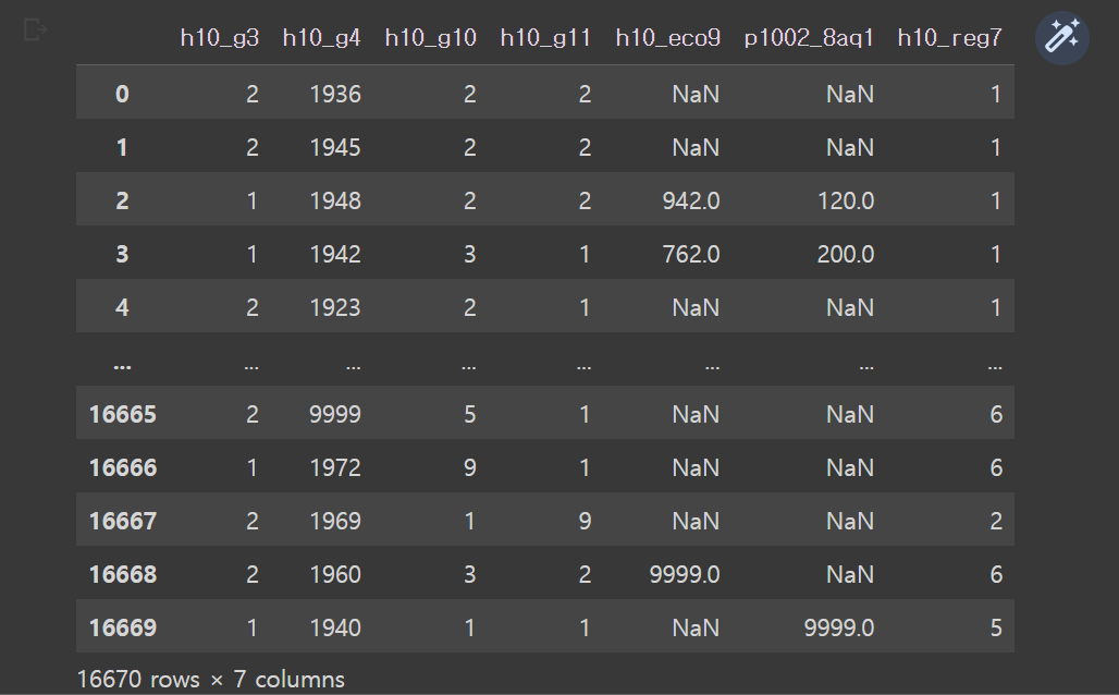
# 사본 저장
welfare = raw_welfare.copy()
# 데이터 살펴보기
# 데이터 앞부분, 뒷부분 확인
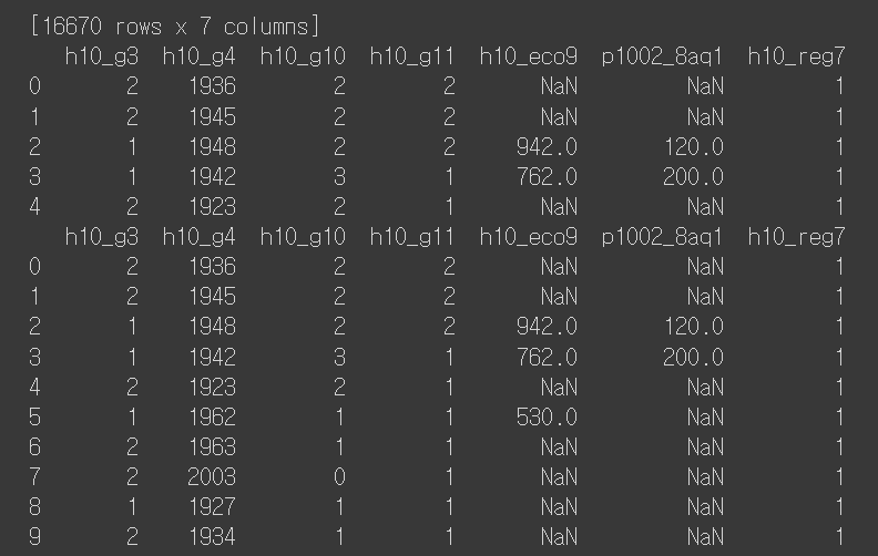
print(welfare) # 데이터프레임은 자동으로 앞부분과 뒷부분을 보여줌
print(welfare.head())
print(welfare.head(10))
print(welfare.tail())
print(welfare.tail(10))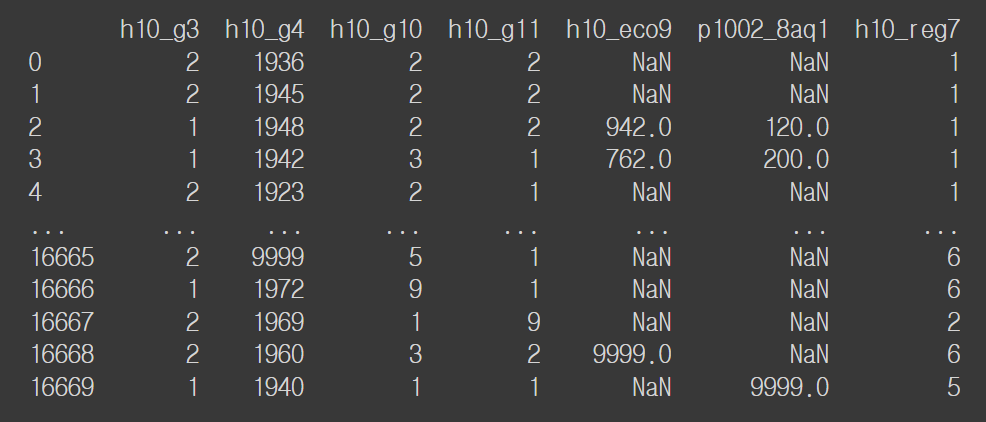
# 행, 열 개수
welfare.shape
----------
(16670, 7)

# 데이터 속성
welfare.info()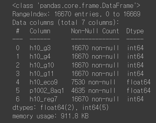
# 데이터 요약 통계량
welfare.describe()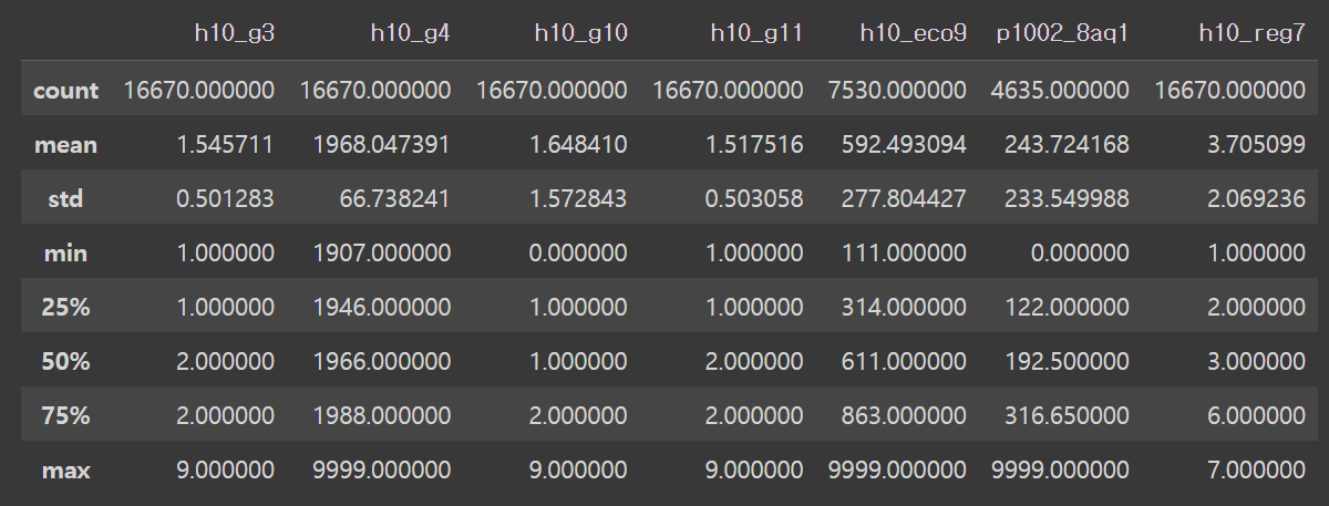
# 데이터 로드
raw_welfare = pd.read_csv('/content/drive/MyDrive/hana1/Data/welfare_2015.csv')
data = raw_welfare.copy()
data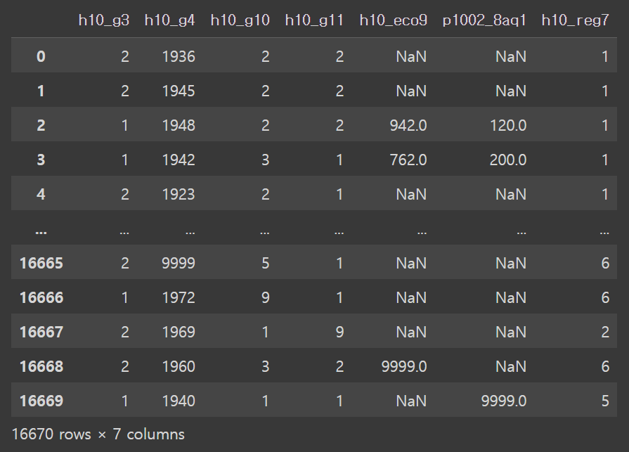
welfare = welfare.rename(columns = {'h10_g3': 'sex',
                                    'h10_g4': 'birth_year',
                                    'h10_g10': 'marital_status',
                                    'h10_g11': 'religion',
                                    'h10_eco9': 'job_code',
                                    'p1002_8aq1': 'income',
                                    'h10_reg7': 'region_code'})

welfare.head()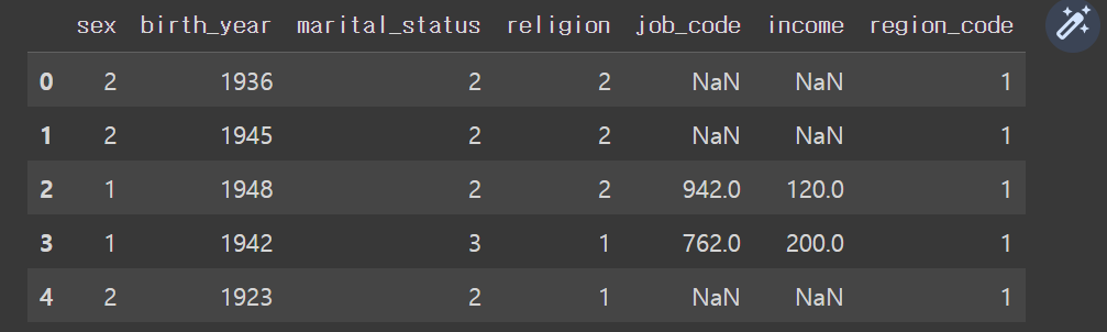
3. 실습
3.1 주제1
3.1.1. 데이터 전처리
# 성별에 따른 월급 차이
# 성별 변수 검토
welfare['sex'].dtypes
-------------------
dtype('int64')

# 범주형 변수 => 빈도표
welfare['sex'].value_counts()
-------------------
2    9089
1    7580
9       1
Name: sex, dtype: int64

# 전처리
# 이상치, 결측치 확인
welfare['sex'].value_counts(dropna = False)
# 9 => 모름/미응답 등으로 이상치 => NaN
# NaN => 현재 없음
-----------------
2    9089
1    7580
9       1
Name: sex, dtype: int64

# 9 => 모름/미응답 등으로 이상치 => NaN
welfare['sex'] = np.where(welfare['sex'] == 9, np.nan, welfare['sex'])

# 이상치, 결측치 확인
welfare['sex'].value_counts(dropna = False)
----------------
2.0    9089
1.0    7580
NaN       1
Name: sex, dtype: int64

# 결측치 확인
welfare['sex'].isnull().sum()
----------------
1

# 1 => 남자, 2 => 여자, NaN => NaN
welfare['sex'] = np.where(welfare['sex'].isnull() == True, np.nan,
                          np.where(welfare['sex'] == 1, 'male', 'female'))

# 이상치, 결측치 확인
welfare['sex'].value_counts(dropna = False)
----------------
female    9089
male      7580
nan          1
Name: sex, dtype: int64

# 결측치 확인
welfare['sex'].isnull().sum()
---------------
0

# 문자열 nan 을 NaN 으로 변환
welfare['sex'] = np.where(welfare['sex'] == "nan", np.nan, welfare['sex'])
# 이상치, 결측치 확인
welfare['sex'].value_counts(dropna = False)
---------------
female    9089
male      7580
**NaN**          1
Name: sex, dtype: int64

# 결측치 확인
welfare['sex'].isnull().sum()
---------------
1

# 빈도 막대그래프
sns.countplot(x = 'sex', data = welfare)
plt.show()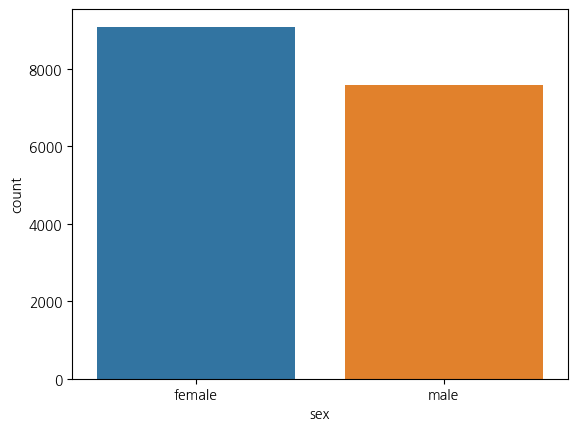
# 월급 변수 검토
welfare['income'].dtypes
-------------
dtype('float64')

# 연속형 변수 => 요약통계량
welfare['income'].describe()
-------------
count    4635.000000
mean      243.724168
std       233.549988
min         0.000000
25%       122.000000
50%       192.500000
75%       316.650000
max      9999.000000
Name: income, dtype: float64


# 전처리
# 이상치, 결측치 확인
welfare['income'].value_counts(dropna = False)
# 9999 => 모름/미응답 등으로 이상치 => NaN
# NaN => 12035개
--------------------
NaN        12035
20.00        136
150.00       128
200.00        91
250.00        74
           ...
392.70         1
515.00         1
397.18         1
304.16         1
9999.00        1
Name: income, Length: 1769, dtype: int64

welfare['income'].describe()
# 0 => NaN
---------------
count    4635.000000
mean      243.724168
std       233.549988
min         0.000000
25%       122.000000
50%       192.500000
75%       316.650000
max      9999.000000
Name: income, dtype: float64


# 9 => 모름/미응답 등으로 이상치 => NaN
welfare['income'] = np.where(welfare['income'] == 9999, np.nan, welfare['income'])

# 이상치, 결측치 확인
welfare['income'].value_counts(dropna = False)
# NaN => 12036개
------------------
NaN       12036
20.00       136
150.00      128
200.00       91
250.00       74
          ...
515.00        1
397.18        1
304.16        1
487.50        1
187.66        1
Name: income, Length: 1768, dtype: int64

# 0 => NaN
welfare['income'] = np.where(welfare['income'] == 0, np.nan, welfare['income'])

# 이상치, 결측치 확인
welfare['income'].value_counts(dropna = False)
# NaN => 12050개
--------------
NaN       12050
20.00       136
150.00      128
200.00       91
250.00       74
          ...
515.00        1
397.18        1
304.16        1
487.50        1
187.66        1
Name: income, Length: 1767, dtype: int64

# 히스토그램
sns.histplot(x = 'income', data = welfare)
plt.show()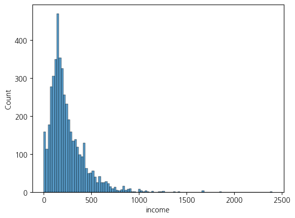
sns.histplot(x = 'income', data = welfare).set(xlim = (0,1000))
plt.show()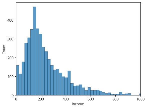
3.1.2.데이터 분석
# 성별에 따른 평균 월급의 차이
welfare.info()
------------------
[50]
0초
12
# 성별에 따른 평균 월급의 차이
welfare.info()
<class 'pandas.core.frame.DataFrame'>
RangeIndex: 16670 entries, 0 to 16669
Data columns (total 7 columns):
 #   Column          Non-Null Count  Dtype
---  ------          --------------  -----
 0   sex             16669 non-null  object
 1   birth_year      16670 non-null  int64
 2   marital_status  16670 non-null  int64
 3   religion        16670 non-null  int64
 4   job_code        7530 non-null   float64
 5   income          4620 non-null   float64
 6   region_code     16670 non-null  int64
dtypes: float64(2), int64(4), object(1)
memory usage: 911.8+ KB

# NaN 이 없는 데이터
welfare.dropna(subset=['sex','income'])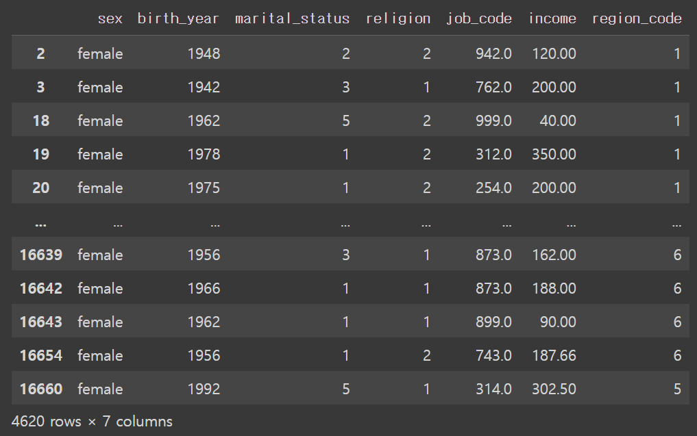
welfare.dropna(subset=['sex','income']).sex.value_counts(dropna=False)
----------------------
female    4620
Name: sex, dtype: int64

welfare.dropna(subset=['sex','income']).income.value_counts(dropna=False)
----------------------
20.00     136
150.00    128
200.00     91
250.00     74
120.00     71
         ...
515.00      1
397.18      1
304.16      1
487.50      1
187.66      1
Name: income, Length: 1766, dtype: int64

welfare.dropna(subset=['sex','income']).income.describe()
-------------------------
count    4620.000000
mean      242.351195
std       184.222067
min         0.460000
25%       123.000000
50%       193.000000
75%       316.700000
max      2400.000000
Name: income, dtype: float64

welfare.dropna(subset=['sex','income']).groupby('sex')
---------------------------
<pandas.core.groupby.generic.DataFrameGroupBy object at 0x7f8a58d8efe0>

welfare.dropna(subset=['sex','income']).groupby('sex').agg({'income': 'mean'})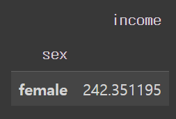
welfare.dropna(subset=['sex','income']).groupby('sex').agg({'income': ['mean', 'std']})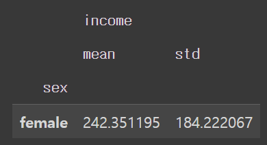
# 변수 이름 만들면서 평균 구하기
welfare.dropna(subset=['sex','income']).groupby('sex').agg(mean_income = ('income','mean'))

# 그룹 이름을 행 인덱스로 사용하지 않고 열로 만들어줌
welfare.dropna(subset=['sex','income']).groupby('sex', as_index=False).agg(mean_income = ('income','mean'))

# 테스트 내용을 종합하여 해결
sex_income = welfare.dropna(subset=['sex','income']) \
                    .groupby('sex', as_index=False) \
                    .agg(mean_income = ('income','mean'))
sex_income

sex_income.iloc[1,1] - sex_income.iloc[0,1]

# 시각화 = 막대그래프
sns.barplot(data=sex_income, x='sex', y='mean_income')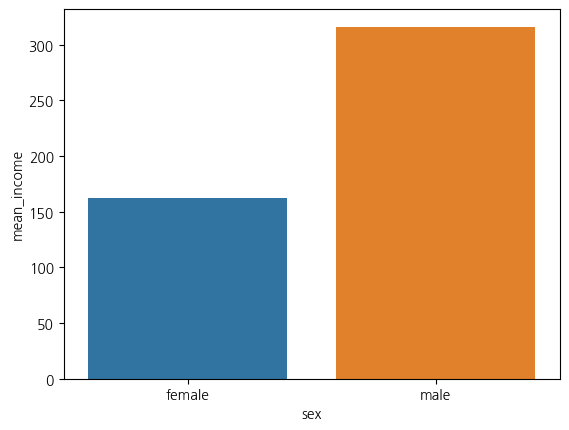
(내가 찾아서 쓴 거)
# 성별에 따른 월급 차이
# 성별 변수 검토
welfare['sex'].dtypes

welfare['sex'] = np.where(welfare['sex'] == 1, 'male', 'female')

sex_income = welfare.dropna(subset=['income']) \
  .groupby('sex', as_index=False) \
  .agg(mean_income=('income', 'mean'))

sex_income
건강보험 청구자료
보험 공단, 심평원에서 제공, 보통 공단 데이터를 많이 사용
심사 데이터: cross sectional data no 연결성
1.남 2. 여자> 범주형
3.2 주제2
3.2.1. 데이터 전처리
welfare.columns
-------------------
Index(['sex', 'birth_year', 'marital_status', 'religion', 'job_code', 'income',
       'region_code'],
      dtype='object')

# 나이와 월급의 관계
# 출생연도 변수 검토
welfare['birth_year'].dtypes
--------------------
dtype('int64')

# 요약통계량
welfare['birth_year'].describe()
-------------------
count    16670.000000
mean      1968.047391
std         66.738241
min       1907.000000
25%       1946.000000
50%       1966.000000
75%       1988.000000
max       9999.000000
Name: birth_year, dtype: float64

# 빈도표
welfare['birth_year'].value_counts()
--------------------
1942    354
1939    300
1940    294
1938    279
1947    269
       ...
1914      1
1911      1
1917      1
1915      1
9999      1
Name: birth_year, Length: 103, dtype: int64

# 전처리
# 이상치, 결측치 확인
welfare['birth_year'].value_counts(dropna = False)
# 9999 => 모름/미응답 등으로 이상치 => NaN
# NaN => 현재 없음
--------------------
[69]
0초
12345
# 전처리
# 이상치, 결측치 확인
welfare['birth_year'].value_counts(dropna = False)
# 9999 => 모름/미응답 등으로 이상치 => NaN
# NaN => 현재 없음
1942    354
1939    300
1940    294
1938    279
1947    269
       ...
1914      1
1911      1
1917      1
1915      1
9999      1
Name: birth_year, Length: 103, dtype: int64

# 9999 => 모름/미응답 등으로 이상치 => NaN
welfare['birth_year'] = np.where(welfare['birth_year'] == 9999, np.nan, welfare['birth_year'])

# 이상치, 결측치 확인
welfare['birth_year'].value_counts(dropna = False)
--------------------
1942.0    354
1939.0    300
1940.0    294
1938.0    279
1947.0    269
         ...
1914.0      1
1911.0      1
1917.0      1
1915.0      1
NaN         1
Name: birth_year, Length: 103, dtype: int64

# 결측치 확인
welfare['birth_year'].isnull().sum()
-------------------
1

# 히스토그램
sns.histplot(x = 'birth_year', data = welfare)
plt.show()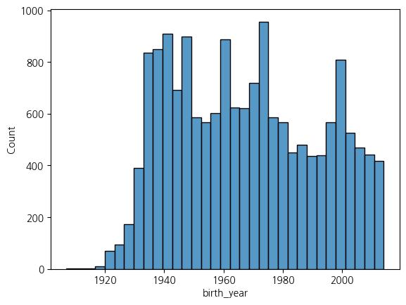
# 나이 변수 만들기
welfare['age'] = 2015 - welfare['birth_year'] + 1

welfare.head()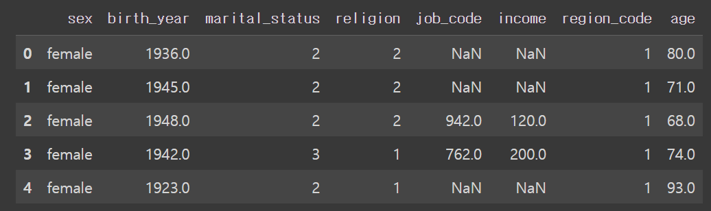
# 이상치, 결측치 확인
welfare['age'].value_counts(dropna = False)
-------------------
74.0     354
77.0     300
76.0     294
78.0     279
69.0     269
        ...
102.0      1
105.0      1
99.0       1
101.0      1
NaN        1
Name: age, Length: 103, dtype: int64

# 결측치 확인
welfare['age'].isnull().sum()
-----------
1

# 요약통계량
welfare['age'].describe()
----------------
count    16669.000000
mean        48.434399
std         24.177789
min          2.000000
25%         28.000000
50%         50.000000
75%         70.000000
max        109.000000
Name: age, dtype: float64

# 히스토그램
sns.histplot(x = 'age', data = welfare)
plt.show()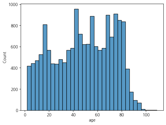
3.2.2. 데이터 분석
welfare.info()
-----------------------
<class 'pandas.core.frame.DataFrame'>
RangeIndex: 16670 entries, 0 to 16669
Data columns (total 7 columns):
 #   Column          Non-Null Count  Dtype
---  ------          --------------  -----
 0   sex             16669 non-null  object
 1   birth_year      16670 non-null  int64
 2   marital_status  16670 non-null  int64
 3   religion        16670 non-null  int64
 4   job_code        7530 non-null   float64
 5   income          4620 non-null   float64
 6   region_code     16670 non-null  int64
dtypes: float64(2), int64(4), object(1)
memory usage: 911.8+ KB

# 나이에 따른 평균 월급 차이
age_income = welfare.dropna(subset=['age','income']) \
                    .groupby('age', as_index=False) \
                    .agg(mean_income = ('income','mean'))
age_income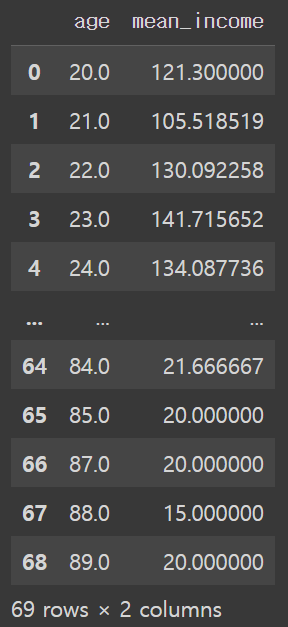
age_income[age_income['mean_income'] == age_income['mean_income'].max()]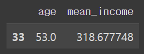
# 시각화 = 선 그래프
sns.lineplot(x = 'age', y = 'mean_income', data = age_income)
plt.show()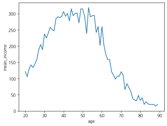
2.4 중간 데이터 저장
welfare.to_csv('/content/drive/MyDrive/hana1/Data/welfare_2015_0608.csv')
!굉장나 엄청해!