Python | matplotlib 시각화.

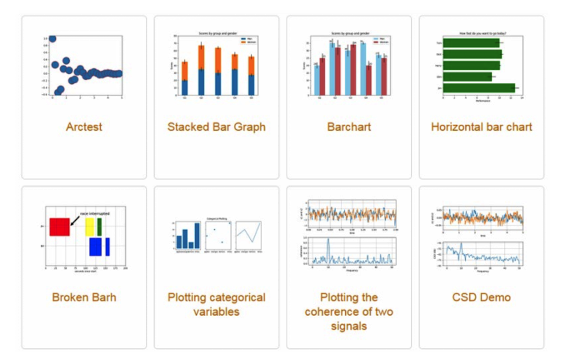
matplotlib 시각화.

• Matplotlib는 데이터 시각화와 2D 그래프 플롯에 사용되는 파이썬 라이브러리.

Matplotlib 기본 사용.

• matplotlib.pyplot
• 기본 그래프

  • import matplotlib.pyplot as plt

    import matplotlib.pyplot as plt
    
    plt.plot([1,2,3,4]) # x 값 자동 완성.
    plt.ylabel('y-label')
    plt.show()

• 기본 그래프

  import matplotlib.pyplot as plt
  
  plt.plot([1,2,3,4], [1,4,9,16]) # x, y 지정
  plt.show()

• 레이블 설정.

  import matplotlib.pyplot as plt
  
  plt.plot([1,2,3,4], [1,4,9,16])
  plt.xlabel('X-label')
  plt.ylabel('Y-label')
  plt.show()

• matplotlib 축 범위 지정하기.
  • matplotlib.pyplot 모듈의 axis() 함수를 사용.

import matplotlib.pyplot as plt

plt.plot([1,2,3,4], [1,4,9,16]) # x, y 지정.
plt.xlabel('X-label')
plt.ylabel('Y-label')
plt.axis([0, 5, 0, 20])
plt.show()

• Matplotlib 마커 지정하기.
  • 입력이 없으면 디폴트 선은 실선.
  • 마커 형태 지정.

import matplotlib.pyplot as plt

plt.plot([1,2,3,4], [1,4,9,16], 'bo') # x, y 지정.
plt.xlabel('x-label')
plt.ylabel('y-label')
plt.axis([0, 5, 0, 20])
plt.show()

• matplotlib 색상 지정하기.
  • 그래프 선 색 지정.

import matplotlib.pyplot as plt

plt.plot([1,2,3,4], [1,4,9,16], 'r')
plt.plot([1,2,3,4], [1,3,5,7], 'violet')

plt.xlabel('X-label')
plt.ylabel('Y-label')
plt.axis([0, 5, 0, 20])
plt.show()

• 스타일 지정.

  • x, y 값 인자에 대해 선의 색상과 형태를 지정하는 포맷 문자열을 세번째 인자에 입력.

    import matplotlib.pyplot as plt
    
    plt.plot([1,2,3,4], [1,4,9,16], 'ro')
    plt.axis([0,6,0,20])
    plt.show()

• 여러 개의 그래프 그리기.

  • matplotlib에서는 일반적으로 Numpy 어레이를 이용.

  • Numpy 어레이를 사용하지 않더라도 모든 시퀀스는 내부적으로 Numpy 어레이로 변환.

    import matplotlib,pyplot as plt
    import numpy as np
    
    t = np.arange(0., 5., 0.2)
    
    plt.plot(t, t, 'r--', t, t**2, 'bs', t, t**3, 'g^')
    plt.show()

• Matplotlib 그래프 영역 채우기.

  • 그래프의 특정 영역을 색상으로 채워서 강조.
    - fill_between()
    - fill_betweenx()
    - fill()

    import matplotlib.pyplot as plt
    
    x = [1,2,3,4]
    y = [1,4,9,16]
    
    plt.plot(x, y)
    plt.xlabel('X-label')
    plt.ylabel('Y-label')
    plt.fill_between(x[1:3], y[1:3], alpha = 0.5)
    
    plt.show()

• Matplotlib 그래프 영역 채우기.

  • 그래프의 특정 영역을 색상으로 채워서 강조.
    - fill_between()
    - fill_betweenx()
    - fill()

    import matplotlib.pyplot as plt
    
    x = [1,2,3,4]
    y = [1,4,9,16]
    
    plt.plot(x, y)
    plt.xlabel('X-label')
    plt.ylabel('Y-label')
    plt.fill_betweenx(y[2:4], x[2:4], alpha = 0.5)
    
    plt.show()

• Matplotlib 그래프 영역 채우기 - 두 그래프 사이 영역 채우기.

  import matplotlib .pyplot as plt
  
  x = [1,2,3,4]
  y1 = [1,4,9,16]
  y2 = [1,2,4,8]
  
  plt.plot(x, y1)
  plt.plot(x, y2)
  plt.xlabel('X-label')
  plt.ylabel('Y-label')
  plt.fill_between(x[1:3], y1[1:3], y2[1:3], color = "lightgray", alpha = 0.5)
  
  plt.show()

  matplotlib 그래프 영역 채우기 - 임의의 영역 채우기.

  import matplotlib.pyplot as plt
  
  x = [1,2,3,4]
  y1 = [1,4,9,16]
  y2 = [1,2,4,8]
  
  plt.plot(x, y1)
  plt.plot(x, y2)
  plt.xlabel('X-label')
  plt.ylabel('Y-label')
  plt.fill([1.9, 1.9, 3.1, 3.1], [2, 5, 11, 8],
  color = 'lightgray', alpha = 0.5)
  
  plt.show()

• matplotlib 눈금 표시하기.
  • 틱은 그래프의 축에 간격을 구분하기 위해 표시하는 눈금.
  • matplotlib.pyplot 모듈의 xticks(), yticks(), tick_params() 함수 이용.

import matplotlib.pyplot as plt
import numpy as np

a = np.arange(0, 2, 0.2)

plt.plot(a, a, 'bo')
plt.plot(a, a**2, color = 'red' marker = '*', linewidth = 2)
plt.plot(a, a**3, color = 'springgreen' marker = '^', markersize = 9)
plt.xticks([0, 1, 2])
plt.yticks(np.arange(1, 6))

plt.show()

matplotlib 타이틀 설정.

import matplotlib.pyplot as plt
import numpy as np

a = np.arnage(0, 2, 0.2)

plt.plot(a, a, 'bo')
plt.plot(a, a**2, color = 'red', marker = '*', linewidth = 2)
plt.plot(a, a**3, color = 'springgreen' marker = '^', markersize = 9)
plt.xticks([0, 1, 2])
plt.yticks(np,arange(1, 6))
plt.title('Title test')

plt.show()

matplotlib 막대 그래프 그리기.

• matplotlib.pyplot 의 bar() 함수 이용.

import matplotlib.pyplot as plt
import numpy as np

x = np.arange(3)
years = ['2017', '2018', '2019']
values = [100, 400, 900]

plt.bar(x.values)
plt.xticks(x, years)
plt.show()

• 스타일 지정.

plt.bar(x, values, width = 0.6,
align = 'edge', color = 'springgreen',
edgecolor = 'gray', linewidth = 3, tick_label = years, log=True)

width는 막대 너비. 디폴트 값 0.8

align는 틱과 막대의위치 조절. 디폴트 값은 ‘center’, ‘edge’로 설정하면 막대의 왼쪽 끝에 x_tick 표시.

color는 막대의 색 지정.

edgecolor는 막대의 테두리 색 지정.

linewidth는 테두리의 두께 지정.

tick_label을 어레이 형태로 지정하면, 틱에 어레이의 문자열을 순서대로 나타낼 수 있음.

log = True로 설정하면, y축이 로그 스케일로 표시.

matplotlib 수평 막대 그래프 그리기.

import matplotlib as plt
import numpy as np

y = np.arnage(3)
years = ['2017', '2018', '2019']
values = [100, 400, 900]

plt.barh(y, values, height = 0.6, align = 'edge', color = 'springgreen',
edgecolor = 'gray', linewidth = 3, ticl_label = years, log = False)
plt.show()

matplotlib 산점도 그리기.

• 산점도는 두 변수의 상관 관계를 직교 좌표계의 평면에 데이터를 점으로 표현하는 그래프.
• matplotlib.pyplot 모듈의 scatter() 함수 이용.

import matplotlib.pyplot as plt
import numpy as np

np.random.seed(19680801)

N = 50
x = np.random.rand(N)
y = np.rnadom.rand(N)
colors = np.random.rand(N))**2
area = (30 * np.random.rand(N)) ** 2

plt.scatter(x, y, s = area, c = colors, alpha = 0.5)
plt.show()

matplotlib 히스토그램 그리기.

• 히스토그램은 도수분포표를 그래프로 나타낸 것으로서, 가로축은 계급, 세로축은 도수 (횟수나 개수 등)를 나타냄.
• matplotlib.pyplot 모듈의 hist() 함수를 이용.

import matplotlib.pyplot as plt

weight = [68, 81, 64, 56, 78, 74, 61, 77, 66, 68, 59, 71, 80, 59, 67, 81, 69, 73, 69, 74, 70, 65]
plt.hist(weight)
plt.show()

• 여러 개 히스토그램.

import matplotlib.pyplot as plt
import numpy as np

a = 2.0 * np.random.rnadn(10000) + 1.0
b = np. rnadom.standard_normal(10000)
c = 20.0 * np.random.rand(5000) = 10.0

plt.hist(a, bins = 100, density = True, alpha = 0.7, histtype = 'step')
plt.hist(b, bins = 50, density = True, alpha = 0.5, histtype = 'stepfilled')
plt.hist(c, bins = 100, density = True, alpha = 0.9, histtype = 'step')
plt.show()

matplotlib 에러바 그리기.

• 에러바(Errorbar, 오차 막대)는 데이터의 편차를 표시하기 위한 그래프 형태.
• matplotlib.pyplot 모듈의 errorbar() 함수 이용.

import matplotlib.pyplot as plt

x = [1,2,3,4]
y = [1,4,9,16]
yerr = [2.3, 3.1, 1.7, 2.5]

plt.errorbar(x, y, yerr = yerr)
plt.show()

• 비대칭 편차 나타내기.

import matplotlib.pyplot as plt

x = [1,2,3,4]
y = [1,4,9,16]
yerr = [(2.3, 3.1, 1.7, 2.5), (1.1, 2.5, 0.9, 3.9)]

plt.errorbar(x, y, yerr= yerr)
plt.show()

matplotlib 파이차트 그리기.

• 범주별 구성 비율을 원형으로 표현한 그래프.
• matplotlib.pyplot 모듈의 pie()함수 이용.

import matplotlib.pyplot as plt

ratio = [34, 32, 16, 18]
labels = ['Apple', 'Banana', 'Melon', 'Grapes']

plt.pie(ratio, labels = labels, autopct = '%1.f%%')
plt.show()

• 시작 각도와 방향 설정.

plt.pie(ratio, labels = labels, autopct = '%.1f%%', startangle = 260,
counterclock = False)

matplotlib 파이차트 그리기.

• 그림자 나타내기.
• 색상지정.

import matpotlib.pyplot as plt

ratio = [34, 32, 16, 18]
labels = ['Apple', 'Banana', 'Melon', 'Grapes']
explode = [0.05, 0.05, 0.05, 0.05]
colors = ['silver', 'gold', 'whitesmoke', 'lightgray']

plt.pie(ratio, labels = labels, autopct = '%.1f%%',
startangle = 260, counterclock = False, explode = explode,
shadow = True, colors = colors)
plt.show()

xml의 이해.

XML의 개념.

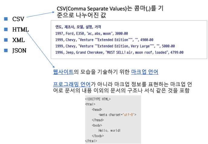
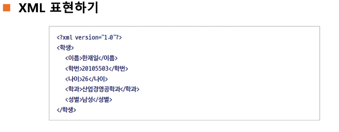
• XML은 확장적인 마크업 언어라는 뜻으로, 데이터의 구조와 의미를 설명하는 태그를 사용하여 어떤 데이터의 속성과 값을 표현하는 언어.
• 시작 태그와 종료태그 사이에 값이 있고, 그 값은 태그의 이름으로 만들어진 속성에 대한 값.

XML의 개념.

• 정보의 구조에 대한 정보인 스키마와 DTD 등으로 정보에 대한 정보가 표현.
• 용도에 따라 다양한 형태로 변형 가능.
• 컴퓨터 간에 정보를 주고 받기 위한 유용한 저장방식으로 사용됨.

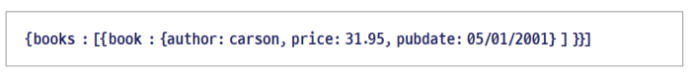
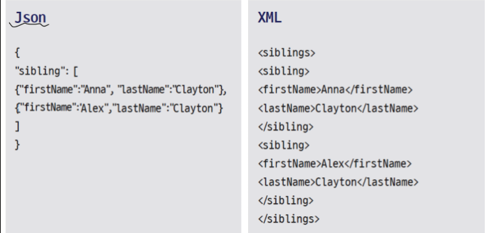
XML 문서.

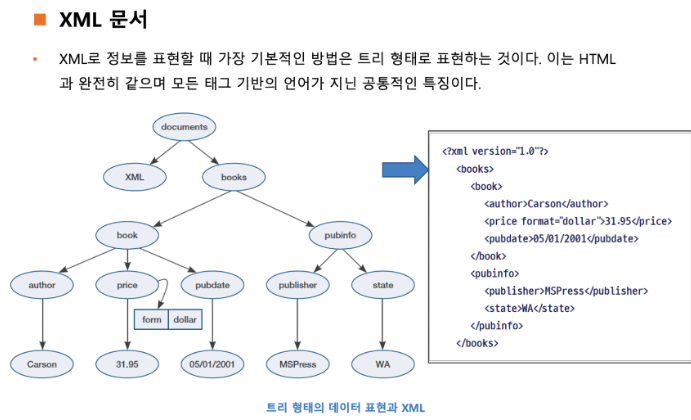
• 간단한 딕셔너리로 생각하면 다음과 같은 방식으로 표현할 수 있다.

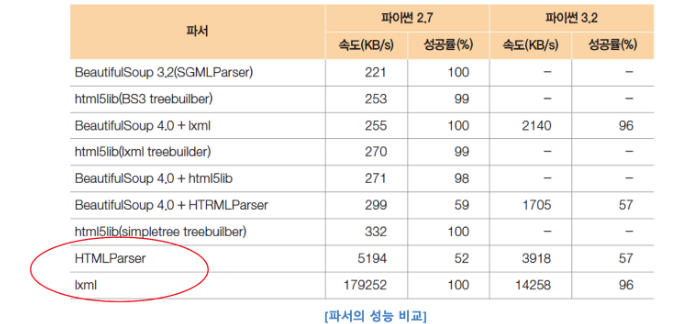
XML Parsing in Python.

• 정규식으로도 파싱 가능.
• 사용하기 쉬운 도구들이 갭발되어 있음.
• 가장 많이 쓰이는 파서는 BeautifulSoup.

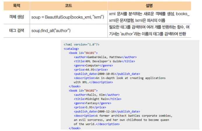
BeautifulSoup 모듈 개요.

• beautifulsoup 모듈은 HTML과 XML 문서들의 구문을 분석하기 위한 파이썬 패키지.
• 전통적인 파이썬 XML 파서(XML Parser)에는 lxml과 htmlslib 드이 있으며, Beautifulsoup모듈은 이를 차용하여 데이터를 쉽고 빠르게 처리함.

BeautifulSoup 모듈 사용법.

from bs4 import BeautifulSoup

with open("../Users/chohyunjun/Desktop/data/books (1).xml", "r", encoding = "utf8")as books_file:
    books_xml = books_file.read()

soup = BeautifulSoup(books_xml, "lxml")

#aouthor가 들어간 모든 요소의 값 추출.
for book_info in soup.find_all("author"):
    print(book_info)
    print(book_info.get_text())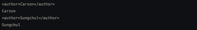

)

PSPTO XML 데이터.

• 미국 특허청의 특허 데이터는 XML 제공됨.
• 특정 특허 XML 문서로부터 필요한 정보 가져오는 실습 : 분석할 특허는 등록번호.

import urllib.request
from bs4 import BeautifulSoup

with open("../Users/chohyunjun/Desktop/data/US08621662-20140107 (1).xml", "r", encoding = "UTF8") as patent_xml:
    xml = patent_xml.read()

soup = BeautifulSoup(xml, "lxml")

invention_title_tag = soup.find("invention-title")
print(invention_title_tag.get_text())

Lab: XML 파싱.

import urllib.request
from bs4 import BeautifulSoup

with open("../Users/chohyunjun/Desktop/data/US08621662-20140107 (1).xml", "r", encoding = 'utf8')as patent_xml:
    xml = patent_xml.read()

soup = BeautifulSoup(xml, "lxml")

invention_title_tag = soup.find("invention-title")
print(invention_title_tag.get_text())

publication_reference_tag = soup.find("publication-reference")
p_document_id_tag = publication_reference_tag.find("document-id")
p_country = p_document_id_tag.find("country").get_text()
p_doc_number = p_document_id_tag.find("doc-number").get_text()
p_kind = p_document_id_tag.find("kind").get_text()
p_date = p_document_id_tag.find("date").get_text()

JSON의 이해.

• JSON의 개념.
• (JAVASCRIPT OBJECT Notation)
• JSON은 XML보다 데이터 용량이 적고 코드로의 전환이 쉽다는 측면에서 XML의 대체로 가장 많이 활용되고 있음.
• JSON은 파이썬의 딕셔너리형과 매우 비슷.
• key:value의 쌍으로 구성되어 있음.

JSON과 XML.

• XML과 비교할 때 JSON의 장점.
• 간결한 코드.
• 쉬운 코드의 전환.
• 코드의 간결함 때문에 용량의 절약(가장 큰 장점)

JSON IN PYTHON.

• JSON 모듈을 사용하여 손 쉽게 파싱 및 저장 가능.
  • PYTHON은 기본적으로 JSON 표준 라이브러리(json) 제공.
  • ‘import json’을 사용하여 JSON 라이브러리 사용.
  • JSON 라이브러리를 사용하여 PYTHON 타입의 Object를 JSON 문자열로 변경할 수 있고(JSON인코딩), 또한 JSON 문자열을 다시 Python 타입으로 변환할 수 있음.(JSON 디코딩)
  • 데이터 저장 및 읽기는 dict type과 상호 호환 가능.
  • 웹에서 제공하는 API는 대부분 정보 교환 시 JSON 활용.
  • 페이스북, 트위터, GITHUB 등 거의 모든 사이트.
  • 각 사이트 마다 Developer API의 활용법을 찾아 사용.

Lab : JSON 데이터 분석 - 읽기.

• JSON 읽기.
  • 파이썬에서 JSON dmf tkdydgkrl dnlgotjsms .Json 모듈 이용. Json 데이터 포맷은 데이터 저장 및 읽기가 딕셔너리형과 완벽히 상호 호환되어, 딕셔너리형에 익숙한 사용자가 매우 쉽게 사용할 수 있다는 장점이 있음.
  • JSON을 읽기 위해서는 JSON 파일의 구조를 확인한 후, JSON 모듈로 읽고 딕셔너리형처럼 처리한다.

Sample data(json_example.json)

• 앞 sample data 에는 ‘employees’ 아래에 3개의 데이터가 있다.
• 파이썬으로 읽어 오기 위해 다음과 같이 입력.

import json
with open("json_example.json","r",encoding = "utf8") as f:
	contents = f.read()
	json_data = json.loads(contents)
	print(json_data["employees"])

• JSON 읽기.

  • 1행에서 JSON 모듈을 호출.

  • 3행에서 open() 함수를 사용하여 파일 내용을 가져옴.

  • 4행에서 문자열형으로 변환하여 처리.

  • 5행에서는 loads() 함수를 사용하여 해당 문자열을 딕셔너리형처럼 변환.

  • 6행에서 테스트로 json_data[”employees”]를 출력.

    읽기 - request 모듈 사용.

    import requests
    url = '웹사이트 json 파일'
    
    data =requests.get(url).json()
    
    <예제>
    import requests
    url = '.....'
    
    data = requests.get(url).json()
    print(data)

    JSON 쓰기.

  • 딕셔너리형으로 구성된 데이터를 json형태의 파일로 변환하는 과정에 대해 알아보자.

    import json
    
    dict_data = {'Name' : 'Zara', 'Age':7, 'Class':'First'}
    
    with open("data.json","w") as f:
    	json.dump(dict_data, f)

    → Json을 파일 작성.

  • 3행처럼 데이터를 저장한 딕셔너리형 생성.

  • 6행에서 Json.dump() 함수를 사용하여 데이터 저장. 이때 인수는 딕셔너리형 자료와 파일 객체.

  • 실행 결과, 작업 폴더에 ‘data.json’ 파일.