https://ocw.mit.edu/courses/18-06-linear-algebra-spring-2010/video_galleries/video-lectures/
먼저 강의에서 다음과 같은 내용을 정리한다.
<orthonormal vectors > q i T q j = { 0 , if i ≠ j 1 , if i = j \text{<orthonormal vectors\>> } \\ q_i^Tq_j= \begin{cases} 0, & \text{if } i \ne j \\ 1, & \text{if } i = j \end{cases} <orthonormal vectors > q i T q j = { 0 , 1 , if i = j if i = j orthogonal basis : q 1 , q 2 , . . . , q n orthogonal matrix : Q \text{orthogonal basis} : q_1,q_2,...,q_n \\ \text{orthogonal matrix} : Q orthogonal basis : q 1 , q 2 , . . . , q n orthogonal matrix : Q how can A → Q ? → “Gran-Schmidt" \text{how can $A \rightarrow Q$ ?} \rightarrow \text{``Gran-Schmidt"} how can A → Q ? → “Gran-Schmidt" 즉, orthonomal vector의 조건은 위와 같고, 이를 orthogonal basis로 구성하는 orthogonal matrix Q를 "Gran-Shcmidt" 방식으로 구할 수 있다는 것이다.
예시와 함께 보자.
Q = [ ∣ ∣ ∣ ∣ q 1 q 2 . . . q n ∣ ∣ ∣ ∣ ] Q= \begin{bmatrix} | & | & | & | \\ q_1 & q_2 & ... & q_n \\ | & | & | & | \\ \end{bmatrix} Q = ⎣ ⎢ ⎡ ∣ q 1 ∣ ∣ q 2 ∣ ∣ . . . ∣ ∣ q n ∣ ⎦ ⎥ ⎤ Q T Q = [ − ( q 1 ) T − − ( q 2 ) T − . − ( q n ) T − ] [ ∣ ∣ ∣ ∣ q 1 q 2 . . . q n ∣ ∣ ∣ ∣ ] = [ 1 0 0 1 0 . . . . 0 1 ] = I Q^TQ = \begin{bmatrix} -(q_1)^T- \\ -(q_2)^T- \\ . \\ -(q_n)^T- \\ \end{bmatrix} \begin{bmatrix} | & | & | & | \\ q_1 & q_2 & ... & q_n \\ | & | & | & | \\ \end{bmatrix} = \begin{bmatrix} 1 & \ & \ & 0 \\ 0 & 1 & \ & 0 \\ . & . & . & . \\ 0 & \ & \ & 1 \\ \end{bmatrix} = I Q T Q = ⎣ ⎢ ⎢ ⎢ ⎡ − ( q 1 ) T − − ( q 2 ) T − . − ( q n ) T − ⎦ ⎥ ⎥ ⎥ ⎤ ⎣ ⎢ ⎡ ∣ q 1 ∣ ∣ q 2 ∣ ∣ . . . ∣ ∣ q n ∣ ⎦ ⎥ ⎤ = ⎣ ⎢ ⎢ ⎢ ⎡ 1 0 . 0 1 . . 0 0 . 1 ⎦ ⎥ ⎥ ⎥ ⎤ = I 위 수식을 통해서 Q T Q = I Q^TQ=I Q T Q = I
그리고 다음과 같이 정리할 수 있다.
If Q is square then Q T Q = I tell us Q T = Q − 1 \text{If $Q$ is square then $Q^TQ=I$ tell us $Q^T=Q^{-1}$} If Q is square then Q T Q = I tell us Q T = Q − 1 Ex. : Q = [ 0 0 1 1 0 0 0 1 0 ] , Q = [ c o s θ − s i n θ s i n θ c o s θ ] , Q = 1 2 [ 1 1 1 − 1 ] Q = 1 2 [ 1 1 1 1 1 − 1 1 − 1 1 1 − 1 − 1 1 − 1 − 1 1 ] \text{Ex.} : Q=\begin{bmatrix}0 & 0 & 1 \\1 & 0 & 0 \\0 & 1 & 0 \\\end{bmatrix}, Q=\begin{bmatrix}cos\theta & -sin\theta \\ sin\theta & cos\theta\end{bmatrix}, Q=\frac{1}{\sqrt{2}}\begin{bmatrix}1 & 1 \\ 1 & -1\end{bmatrix} \\ Q=\frac{1}{2}\begin{bmatrix}1 & 1 & 1 & 1\\ 1 & -1 & 1 & -1 \\ 1 & 1 & -1 & -1\\ 1 & -1 & -1 & 1\\ \end{bmatrix} Ex. : Q = ⎣ ⎢ ⎡ 0 1 0 0 0 1 1 0 0 ⎦ ⎥ ⎤ , Q = [ c o s θ s i n θ − s i n θ c o s θ ] , Q = 2 1 [ 1 1 1 − 1 ] Q = 2 1 ⎣ ⎢ ⎢ ⎢ ⎡ 1 1 1 1 1 − 1 1 − 1 1 1 − 1 − 1 1 − 1 − 1 1 ⎦ ⎥ ⎥ ⎥ ⎤ 그렇다면 Q Q Q
Q = 1 3 [ 1 − 2 2 − 1 2 2 ] → 1 3 [ 1 − 2 2 2 − 1 2 2 2 1 ] Q= \frac{1}{3} \begin{bmatrix} 1 & -2 \\ 2 & -1 \\ 2 & 2 \\ \end{bmatrix} \rightarrow \frac{1}{3} \begin{bmatrix} 1 & -2 & 2 \\ 2 & -1 & 2 \\ 2 & 2 & 1 \\ \end{bmatrix} Q = 3 1 ⎣ ⎢ ⎡ 1 2 2 − 2 − 1 2 ⎦ ⎥ ⎤ → 3 1 ⎣ ⎢ ⎡ 1 2 2 − 2 − 1 2 2 2 1 ⎦ ⎥ ⎤ 위 과정은 Gram-Schmidt의 개략적인 과정을 의미한다.
Suppose : Q has orthonormal columns. proejct onto it’s column space. \text{Suppose : $Q$ has orthonormal columns.} \\ \text{proejct onto it's column space.} Suppose : Q has orthonormal columns. proejct onto it’s column space. p = Q ( Q T Q ) − 1 Q T = Q I − 1 Q T = Q Q T (=1 if Q is square) p=Q(Q^TQ)^{-1}Q^T=QI^{-1}Q^T=QQ^T \text{(=1 if Q is square)} p = Q ( Q T Q ) − 1 Q T = Q I − 1 Q T = Q Q T (=1 if Q is square) ( Q Q T ) ( Q Q T ) = Q I Q T = Q Q T (QQ^T)(QQ^T)=QIQ^T=QQ^T ( Q Q T ) ( Q Q T ) = Q I Q T = Q Q T A T A x ^ = A T b A → Q A^T A \hat x=A^Tb \\ A \rightarrow Q A T A x ^ = A T b A → Q Q T Q x ^ = Q T b Q^TQ\hat x=Q^Tb Q T Q x ^ = Q T b I x ^ = Q T b I\hat x=Q^Tb I x ^ = Q T b ∴ x ^ = Q T b \therefore \hat x=Q^Tb ∴ x ^ = Q T b ∴ x ^ i = q i T b \therefore \hat x_i=q_i^Tb ∴ x ^ i = q i T b 그럼 이제 위 식을 이용해서 Gram-Schmidt를 적용하는 절차를 알아보자.
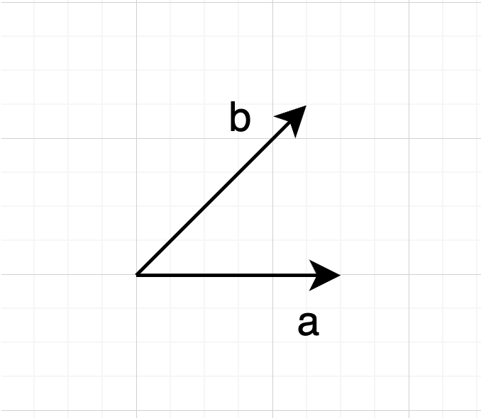
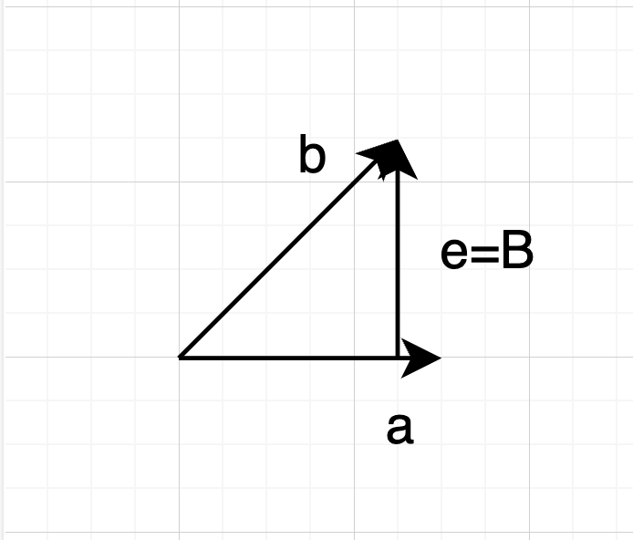
Gram-Schmidt \text{Gram-Schmidt} Gram-Schmidt (independent vectors) a , b → (orthogonal vectors) A , B → orthonormal vectors q 1 = A ∣ ∣ A ∣ ∣ , q 2 = B ∣ ∣ B ∣ ∣ \text{(independent vectors) $a, b$} \rightarrow \text{(orthogonal vectors) $A,B$} \\ \rightarrow \text{orthonormal vectors $q_1=\frac{A}{||A||}$, $q_2=\frac{B}{||B||}$} (independent vectors) a , b → (orthogonal vectors) A , B → orthonormal vectors q 1 = ∣ ∣ A ∣ ∣ A , q 2 = ∣ ∣ B ∣ ∣ B a , b a,b a , b A A A a = A a=A a = A B B B A A A B B B e e e
지난 강의에서 배운 projection 방법을 적용하여 B B B
B = b − A T b A T A A B=b-\frac{A^Tb}{A^TA}A B = b − A T A A T b A 또한 다음과 같은 점도 발견할 수 있다.
A T B = A T ( b − A T b A T A A ) = A T b − A T b A T A A T A = A T b − A T b = 0 A^TB=A^T(b-\frac{A^Tb}{A^TA}A)=A^Tb - \frac{A^Tb}{A^TA}A^TA=A^Tb-A^Tb=0 A T B = A T ( b − A T A A T b A ) = A T b − A T A A T b A T A = A T b − A T b = 0 ∴ A T B = 0 → A ⊥ B \therefore A^TB=0 \rightarrow \text{$A \perp B$} ∴ A T B = 0 → A ⊥ B 이렇게 orthogonal vectors를 구한 후, q 1 = A ∣ ∣ A ∣ ∣ q_1=\frac{A}{||A||} q 1 = ∣ ∣ A ∣ ∣ A q 2 = B ∣ ∣ B ∣ ∣ q_2=\frac{B}{||B||} q 2 = ∣ ∣ B ∣ ∣ B
다만 위는 2개의 벡터에 대해서만 적용하였는데, 만약 벡터의 개수가 늘어난다면 어떻게 적용할 수 있을까? 예를 들어 3개의 벡터에 대해서 Gram-Schmidt를 적용한다고 해보자.
independent vectors a , b , c a,b,c a , b , c
orthgonal vectors
A = a A=a A = a B = b − A T b A T A A B=b-\frac{A^Tb}{A^TA}A B = b − A T A A T b A C = c − A T c A T A A − B T c B T B B C=c - \frac{A^Tc}{A^TA}A - \frac{B^Tc}{B^TB}B C = c − A T A A T c A − B T B B T c B
orthnormal vectors
q 1 = A ∣ ∣ A ∣ ∣ q_1=\frac{A}{||A||} q 1 = ∣ ∣ A ∣ ∣ A q 2 = B ∣ ∣ B ∣ ∣ q_2=\frac{B}{||B||} q 2 = ∣ ∣ B ∣ ∣ B q 3 = C ∣ ∣ C ∣ ∣ q_3=\frac{C}{||C||} q 3 = ∣ ∣ C ∣ ∣ C
위와 같이 B B B C C C A A A B B B
예시와 함께 Gram-Schmidit을 적용해보자.
a = [ 1 1 1 ] , b = [ 1 0 2 ] a=\begin{bmatrix} 1 \\ 1 \\ 1 \end{bmatrix}, b=\begin{bmatrix} 1 \\ 0 \\ 2 \end{bmatrix} a = ⎣ ⎢ ⎡ 1 1 1 ⎦ ⎥ ⎤ , b = ⎣ ⎢ ⎡ 1 0 2 ⎦ ⎥ ⎤ A = [ 1 1 1 ] A=\begin{bmatrix}1 \\ 1 \\ 1\end{bmatrix} A = ⎣ ⎢ ⎡ 1 1 1 ⎦ ⎥ ⎤ B = b − A T b A T A A = [ 1 0 2 ] − 3 3 [ 1 1 1 ] = [ 0 − 1 1 ] B=b-\frac{A^Tb}{A^TA}A=\begin{bmatrix} 1 \\ 0 \\ 2 \end{bmatrix}-\frac{3}{3}\begin{bmatrix} 1 \\ 1 \\ 1 \end{bmatrix} = \begin{bmatrix} 0 \\ -1 \\ 1 \end{bmatrix} B = b − A T A A T b A = ⎣ ⎢ ⎡ 1 0 2 ⎦ ⎥ ⎤ − 3 3 ⎣ ⎢ ⎡ 1 1 1 ⎦ ⎥ ⎤ = ⎣ ⎢ ⎡ 0 − 1 1 ⎦ ⎥ ⎤ q 1 = A ∣ ∣ A ∣ ∣ = 1 3 [ 1 1 1 ] q_1=\frac{A}{||A||}=\frac{1}{\sqrt3}\begin{bmatrix} 1 \\ 1 \\ 1 \end{bmatrix} q 1 = ∣ ∣ A ∣ ∣ A = 3 1 ⎣ ⎢ ⎡ 1 1 1 ⎦ ⎥ ⎤ q 2 = B ∣ ∣ B ∣ ∣ = 1 2 [ 0 − 1 1 ] q_2=\frac{B}{||B||}=\frac{1}{\sqrt{2}}\begin{bmatrix} 0 \\ -1 \\ 1 \end{bmatrix} q 2 = ∣ ∣ B ∣ ∣ B = 2 1 ⎣ ⎢ ⎡ 0 − 1 1 ⎦ ⎥ ⎤ ∴ Q = [ 1 / 3 0 1 / 3 − 1 / 2 1 / 3 1 / 2 ] \therefore Q= \begin{bmatrix}1/\sqrt3 & 0 \\ 1/\sqrt3 & -1/\sqrt2\\ 1/\sqrt3 & 1/\sqrt2 \end{bmatrix} ∴ Q = ⎣ ⎢ ⎡ 1 / 3 1 / 3 1 / 3 0 − 1 / 2 1 / 2 ⎦ ⎥ ⎤ 그리고 Gram-Schmidt를 구하는 과정을 다음과 같이 행렬로 표시할 수 있다.
A = Q R ∼ A = L U A=QR \sim A=LU A = Q R ∼ A = L U 즉, A = Q R A=QR A = Q R R R R
A = [ ∣ ∣ a b ∣ ∣ ] = [ ∣ ∣ q 1 q 2 ∣ ∣ ] ⏟ Q R A= \begin{bmatrix} | & | \\ a & b \\ | & | \end{bmatrix} = \underbrace{ \begin{bmatrix} | & | \\ q_1 & q_2 \\ | & | \end{bmatrix}}_Q R A = ⎣ ⎢ ⎡ ∣ a ∣ ∣ b ∣ ⎦ ⎥ ⎤ = Q ⎣ ⎢ ⎡ ∣ q 1 ∣ ∣ q 2 ∣ ⎦ ⎥ ⎤ R 따라서 위에서 R R R
[ a b ] = [ q 1 q 2 ] [ q 1 T a q 1 T b q 2 T a q 2 T b ] ⏟ R \begin{bmatrix} a & b \\ \end{bmatrix} = \begin{bmatrix} q_1 & q_2 \end{bmatrix} \underbrace{ \begin{bmatrix} q_1^Ta & q_1^Tb\\ q_2^Ta & q_2^Tb \end{bmatrix} }_R [ a b ] = [ q 1 q 2 ] R [ q 1 T a q 2 T a q 1 T b q 2 T b ] 그리고 q 2 T a q_2^Ta q 2 T a q 2 q_2 q 2 a = A a=A a = A q 1 T b q_1^Tb q 1 T b b b b q 1 T q_1^T q 1 T A A A A = Q R A=QR A = Q R R R R U U U