Fraud Detection by Unsupervised Learning

jaehyeong.an_·2021년 6월 17일

Intro

금융거래 중 부정하게 사용되는 거래를 부정 거래라고 합니다. 그 중 신용카드 위변조, 도용, 부정거래에 대한 비율은 해마다 증가하고 있는 추세입니다. 아래 표는 연도별 신용카드 부정사용 금액.

따라서, 최근에는 국내 주요 은행들은 FDS(Fraud Detection System)을 도입하여 이러한 부정거래를 막기위해 노력하고 있지만 주로 룰(Rule) 기반으로 사람에 의해 이루어지기 때문에 실시간으로 정확한 탐지가 어려운 상황이라고 합니다.

목표

여기서는 머신러닝을 이용하여, 이러한 부정거래를 탐지해 보고자 합니다. 하지만, 지도학습이 아닌 비지도 학습을 이용합니다. 그 중 이상 탐지(Outlier Detection) 알고리즘을 이용하여 라벨을 통한 학습이 아닌 이상치 데이터 집단을 찾아 그 이상치 집단이 부정거래 데이터와 일치 및 유사한지 알아볼 것입니다.

1. 신용카드 데이터 셋

데이터 셋의 경우 kaggle에서 제공하는 Credit Card Fraud Detection Dataset을 이용하였습니다.
위 데이터 셋은 2013년 9월 유럽의 실제 신용 카드 거래 데이터를 담고 있습니다. 데이터는 총 284,807건이며 그 중 492건만이 부정 거래 데이터 입니다.
즉, 데이터가 매우 불균형(imbalanced) 합니다.

import pandas as pd

df = pd.read_csv('./input/creditcard.csv')
df.head(10)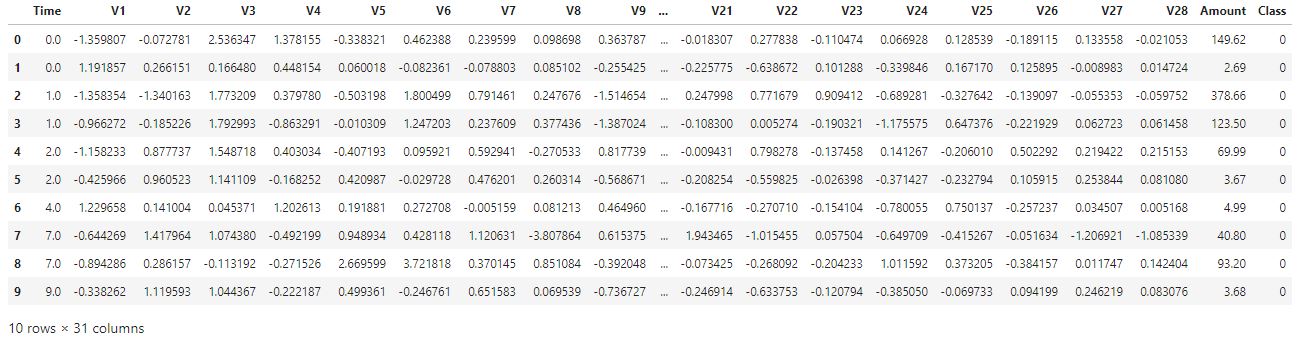

위 데이터 셋은 개인정보 비식별화처리로 인해 칼럼정보를 알 수 없으며, 데이터 또한 스케일(scale) 및 PCA(principal component analysis) 처리 되어있습니다.
총 31개의 칼럼으로 이루어져 있고, Time, Amount, Class를 제외한 모든 칼럼은 비식별화처리 되어있습니다.

df.info()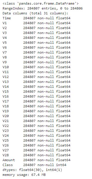

데이터는 총 284,807건이며 null값은 존재하지 않는 정형 데이터 입니다.

2. 데이터 탐색(EDA)

시간(Time)대별 정상/부정 거래 비율

import matplotlib.pyplot as plt

# 시간대별 트랜잭션 양
f, (ax1, ax2) = plt.subplots(2,1, sharex=True, figsize=(12,4))
ax1.hist(df.Time[df.Class==1], bins=50)
ax2.hist(df.Time[df.Class==0], bins=50)

ax1.set_title('Fraud')
ax2.set_title('Normal')
plt.xlabel('Time(in Seconds)'); plt.ylabel('Number of Transactions')
plt.show()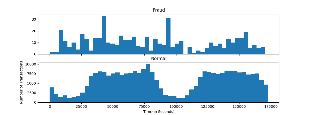

음.. 대체적으로 정상 거래의 경우 시간에 따라 주기적인 반면 부정 거래의 경우 불규칙한 특성을 보입니다.

금액(Amount)대별 정상/부정 거래 비율

import matplotlib.pyplot as plt

# 금액대별 트랜잭션 양
f, (ax1, ax2) = plt.subplots(2,1, sharex=True, figsize=(12,4))
ax1.hist(df.Amount[df.Class==1], bins=30)
ax2.hist(df.Amount[df.Class==0], bins=30)
ax1.set_title('Fraud')
ax2.set_title('Normal')

plt.xlabel('Amount ($)')
plt.ylabel('Number of Transactions')
plt.yscale('log')
plt.show()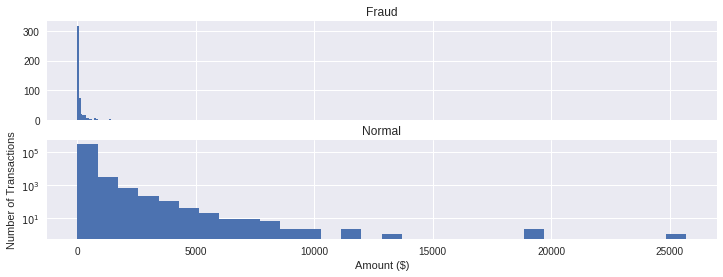

정상 거래의 경우 다양한 금액대에서 발생되지만, 부정 거래의 경우 적은 금액에서 주로 발생하는 것 같습니다.

비식별칼럼 정상/부정거래 비율
특성 차이가 심한 일부 변수만 표시하였습니다.

import matplotlib.pyplot as plt
import seaborn as sns

# 정상/비정산 럼간 값 분포
v_features = df.ix[:,1:29].columns
for cnt, col in enumerate(df[v_features]):
    sns.distplot(df[col][df.Class==1], bins=50)
    sns.distplot(df[col][df.Class==0], bins=50)
    plt.legend(['Y','N'], loc='best')
    plt.title('histogram of feature '+str(col))
    plt.show()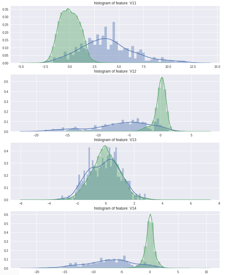

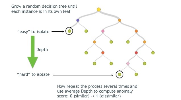
3. Isolation Forest

이상탐지 알고리즘으로는 Isolation Forest 알고리즘을 이용하였습니다. Isolation Forest 는 Tree 기반으로 데이터를 나누어 데이터의 관측치를 고립시키는 알고리즘입니다. 이상 데이터의 경우 root node와 가까운 depth를 가지고, 정상 데이터의 경우 tree의 말단 노드에 가까운 depth를 가집니다.

4. 이상 탐지 알고리즘 적용

Isolation Forest 알고리즘은 현재 scikit-learn에서 제공되고 있으며, 링크를 통해 다큐먼트를 확인하실 수 있습니다.
Isolation Forest는 이상치 점수(outlier score)를 제공합니다. 정상 거래/ 부정 거래에 대한 이상치 점수는 아래와 같습니다.

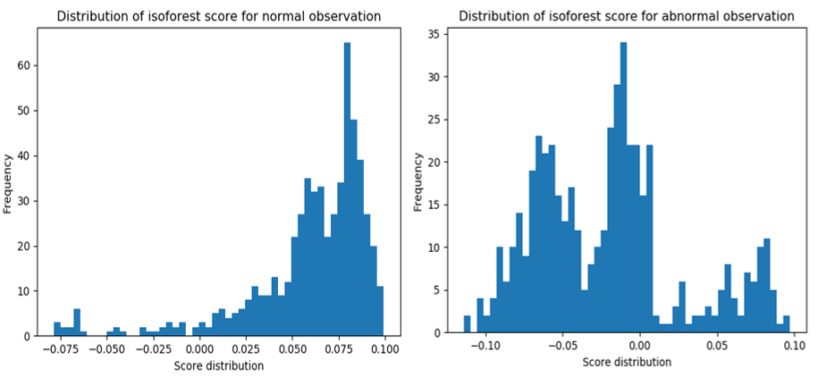
위의 분포를 보았을 때, 정상 / 부정 거래 간 비율이 다르게 나타나는 것을 확인할 수 있습니다.

Python

우선 적용하기에 앞서, 데이터 불균형(Data Imbalance)를 해결하기 위하여, 정상 거래건에 대해 Down sampling을 70% 비율로 진행하였습니다.

import pandas as pd 
from imblearn.under_sampling import RandomUnderSampler

credit_data = pd.read_csv('./data/creditcard.csv')
X = credit_data.drop(['Class'], axis=1)
y = credit_data['Class']
print(Counter(y))	# {0: 284315, 1: 492}

# Under Sampling
sampler = RandomUnderSampler(ratio=0.70, random_state=0)
X, y = sampler.fit_sample(X, y)
print('Class : ',Counter(y))	# {0: 702, 1: 492}
```![](https://velog.velcdn.com/images%2Fjaehyeong%2Fpost%2F3c014a57-6608-4d83-8923-06260ba0ef71%2Fcol.png)

이후, Isolation Forest를 아래와 같은 파라미터를 통해 적용하였습니다.
```python
from sklearn.ensemble import IsolationForest

clf = IsolationForest(n_estimators=300, contamination=0.40, random_state=42)
clf.fit(X)
pred_outlier = clf.predict(X)
pred_outlier = pd.DataFrame(pred_outlier).replace({1:0, -1:1})

n_estimators : 노드 수
contamination : 이상치 비율

이상탐지 예측값은 1이 정상, -1이 이상으로 분류됩니다. 이를 Class 라벨과의 오차를 계산하여야 하기 때문에, 같은 범위로 바꿔주었습니다.

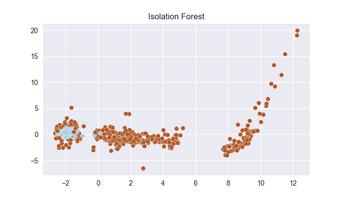
시각화

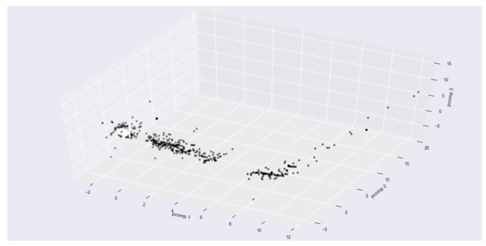
이상탐지 결과를 2d 및 3d로 시각화한 결과 입니다. ( 시각화를 위해 차원을 축소하였습니다.)

import matplotlib.pyplot as plt
from mpl_toolkits.mplot3d import Axes3D

# plot 2d
plt.scatter(X[:,0], X[:,1], c=pred_outlier, cmap='Paired', s=40, edgecolors='white')
plt.title("Isolation Forest")
plt.show()

# plot 3d
fig = plt.figure()
ax = fig.add_subplot(111, projection='3d')
ax.scatter(X[:,0], X[:,1], X[:,2], c=pred_outlier)
ax.set_xlabel('pcomp 1')
ax.set_ylabel('pcomp 2')
ax.set_zlabel('pcomp 3')
plt.show()

2차원 시각화
3차원 시각화

예측 성능

예측값을 실제 부정거래여부 칼럼인 Class와 비교하여 성능을 살펴보겠습니다.
측정 지표로는 Accuracy(정확도), Recall(재현율), Precision(정밀도), F1-score 입니다.

금융 거래에서는 정확도도 물론 중요하지만, 실제 부정거래를 부정거래로 예측하는 비율인 Recall(재현율) 값이 중요하게 여겨집니다.

from sklearn.metrics import confusion_matrix, classification_report, accuracy_score
import itertools

class_name = [0, 1]
def plot_confusion_matrix(classes, pred, y_test, 
                          normalize=False, title='Confusion matrix', cmap=plt.cm.Blues):
    
    cm = confusion_matrix(y_test, pred)
    plt.imshow(cm, interpolation='nearest', cmap=cmap)
    plt.title(title)
    plt.colorbar()
    tick_marks = np.arange(len(classes))
    plt.xticks(tick_marks, classes, rotation=0)
    plt.yticks(tick_marks, classes)
    
    if normalize:
        cm = cm.astype('float') / cm.sum(axis=1)[:, np.newaxis]
    thresh = cm.max() / 2.
    for i, j in itertools.product(range(cm.shape[0]), range(cm.shape[1])):
        plt.text(j, i, cm[i, j],
                 horizontalalignment="center",
                 color="white" if cm[i, j] > thresh else "black")


# 평가
print('confusion matrix\n', confusion_matrix(pred_outlier, y))
print('Accuracy: ',accuracy_score(pred_outlier, y))
print('classification_report\n', classification_report(pred_outlier, y))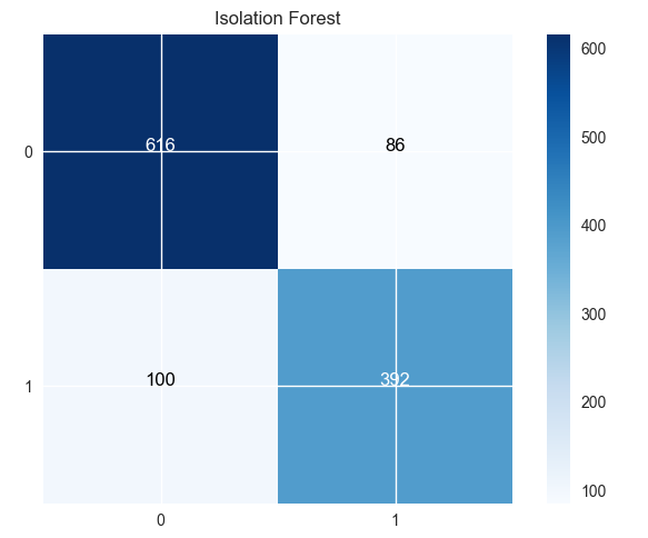
plot_confusion_matrix(class_name, pred_outlier, y, title='Isolation Forest')

Confusion Matrix 결과
Classification report 결과

Accuracy:  0.8442211055276382
classification_report
              precision    recall  f1-score   support

          0       0.88      0.86      0.87       716
          1       0.80      0.82      0.81       478

avg / total       0.85      0.84      0.84      1194

위 결과를 보았을 때, Accuracy 무려 84% 입니다.
Recall 값 또한 82% 로 높은 부정 거래 탐지 정확도를 나타냅니다.