TensorFlow로 CNN 모델 구축

짱아·2025년 8월 20일

AI모델학습

로봇영상처리를 위한 AI모델 학습

목록 보기

5/9

Google에서 만든 딥러닝 프레임워크인 TensorFlow를 활용해서 CNN 모델인 AlexNet과 VGGNet을 만들고 학습시킬 예정이다. 우리가 사용할 데이터셋은 MNIST이다.

https://wikidocs.net/152775
다양한 CNN 네트워크 참조 : https://rubber-tree.tistory.com/120

0. 환경설정

코랩 상단 메뉴에서 런타임 - 런타임 유형 변경을 눌러주세요

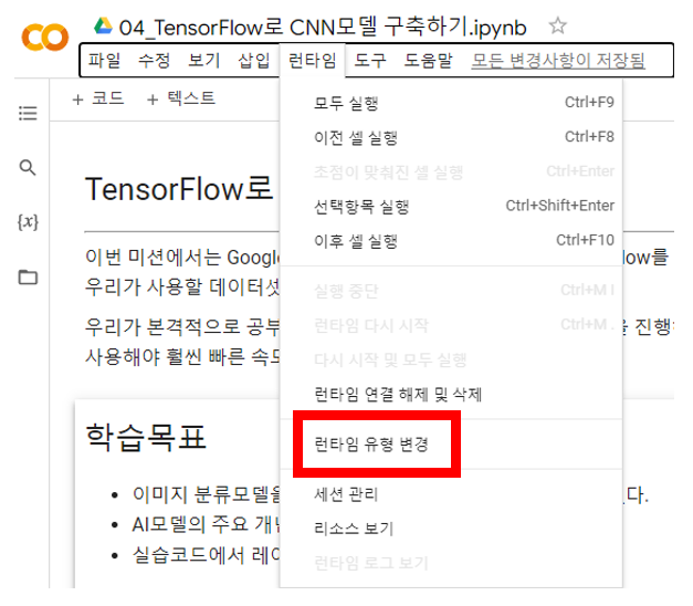
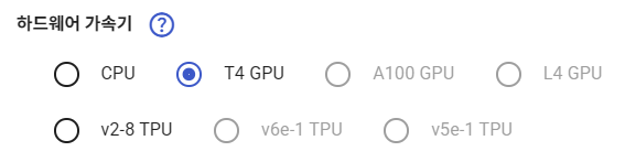
하드웨어 가속기는 T4 GPU로.

MNIST를 활용한 간단한 CNN 모델 만들기

1. MNIST 알아보기

본격적인 미션에 앞서 먼저 MNIST에 대해 알아보도록 하자.
MNIST는 0부터 9까지 숫자 손글씨로 이루어진 데이터셋으로 되어 있다.
28X28사이즈의 60000의 훈련 데이터와 10000개의 테스트 데이터로 구성되어 있다.

x_train.shape == (60000, 28, 28)
x_test.shape == (10000, 28, 28)
y_train.shape == (60000,)
y_test.shape == (10000,)

# 인공지능 학습에 필요한 라이브러리 tensorflow 설치
# 코랩환경에서 불필요
'''
!pip install tensorflow
!pip install numpy
!pip install matplotlib
'''

나는 Colab에서 진행 중이므로 위 코드를 사용하지 않았다.

필요 라이브러리 및 tensorflow 불러오기

import tensorflow as tf
import numpy as np
import matplotlib.pyplot as plt

Keras API를 활용해서 MNIST 불러오기

mnist = tf.keras.datasets.mnist

(train_images, train_labels), (test_images, test_labels) = mnist.load_data()

2. 데이터 확인해보기

train_images 데이터 확인

train_images[2025]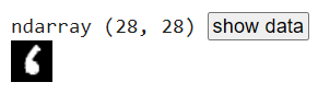

정답 데이터도 확인해보기

train_labels[2025]

시각화해서 확인하기

plt.imshow(train_images[1033],cmap='gray')
print(train_labels[1033],'입니다.')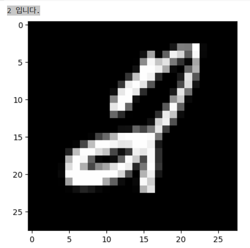

결과는 무슨 숫자인지, 그리고 손글씨 그림을 함께 보여준다.

3. 데이터 전처리 - 정규화하기

최소값과 최대값 확인하기

np.min(train_images), np.max(train_images)

픽셀 값 범위를 [0, 255]에서 [0, 1]로 정규화

train_images = train_images / 255.0
test_images = test_images / 255.0

print('최소값:',np.min(train_images))
print('최대값:',np.max(train_images))

최소값: 0.0
최대값: 1.0 으로 출력된다.

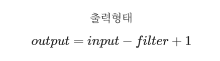
4. 모델 정의 - TensorFlow를 이용한 CNN 모델 만들기

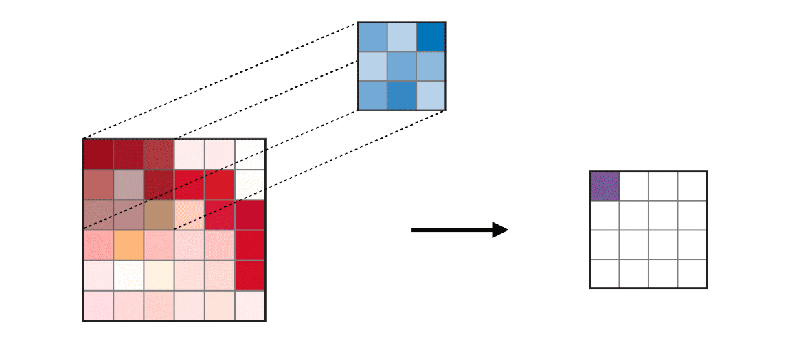
4-1. filters 이해하기

3x3 필터 2개 사용, ReLU 활성화 적용 2D 합성곱층

input_shape = (4, 28, 28, 3)
x = tf.random.normal(input_shape)
# 3x3 필터 2개 사용, ReLU 활성화 적용 2D 합성곱층
y = tf.keras.layers.Conv2D(filters=2, kernel_size=3, activation='relu')(x)

print(y.shape)

결과: (4, 26, 26, 2)

2x2 필터 2개 사용, ReLU 활성화 적용 2D 합성곱층

input_shape = (4, 28, 28, 3)
x = tf.random.normal(input_shape)
# 2x2 필터 2개 사용, ReLU 활성화 적용 2D 합성곱층
y = tf.keras.layers.Conv2D(filters=2, kernel_size=2, activation='relu')(x)

print(y.shape)

결과: (4, 27, 27, 2)

4-2. kernel_size 이해하기

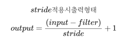
4-3. strides 이해하기

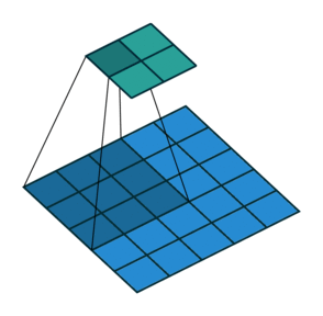
3x3 필터 2개 사용, 스텝사이즈 2, ReLU 활성화 적용 2D 합성곱층

input_shape = (4, 28, 28, 3)
x = tf.random.normal(input_shape)
# 3x3 필터 2개 사용, 스텝사이즈 2, ReLU 활성화 적용 2D 합성곱층
y = tf.keras.layers.Conv2D(filters = 2, kernel_size = 3, activation = 'relu')(x)
print(y.shape)

결과: (4, 26, 26, 2)

3x3 필터 2개 사용, 스텝사이즈 2, ReLU 활성화 적용 2D 합성곱층

input_shape = (4, 28, 28, 3)
x = tf.random.normal(input_shape)
# 3x3 필터 2개 사용, 스텝사이즈 2, ReLU 활성화 적용 2D 합성곱층
y = tf.keras.layers.Conv2D(filters = 2, kernel_size = 3, strides = 2, activation = 'relu')(x)
print(y.shape)

결과: (4, 13, 13, 2)

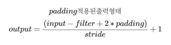
4-4. padding 이해하기

3x3 필터 2개 사용, 패딩 적용, ReLU 활성화 적용 2D 합성곱층

input_shape = (4, 28, 28, 3)
x = tf.random.normal(input_shape)
# 3x3 필터 2개 사용, 패딩 적용, ReLU 활성화 적용 2D 합성곱층
y = tf.keras.layers.Conv2D(filters = 2, kernel_size = 3, activation = 'relu', padding = 'same')(x)
print(y.shape)

결과: (4, 28, 28, 2)

5. [미션 1] TensorFlow로 모델 architecture 직접 만들기

AlexNet

2012년 ImageNet데이터를 기반으로 한 ILSVRC(ImageNet Large Scale Visual Recognition Challenge) 대회에서 우승 -> GPU 사용의 시작, 딥러닝 부응을 가져옴

5-1. 기본 설명

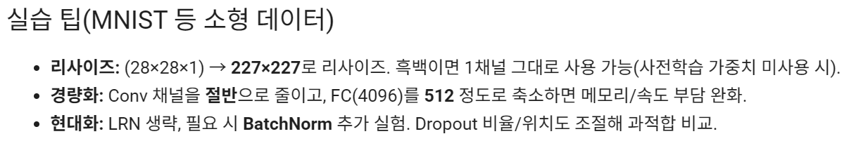
5-2. AlexNet (레이어 구조)

입력 & 전처리
- 입력(28×28×1) → Resizing(227×227×1)
특징 추출부(Convolution + Pooling)
- Conv(96, 11×11, stride=4, ReLU) → 출력: 55×55×96
  - 역할: 아주 큰 11×11 시야로 엣지/윤곽/굵은 질감을 빠르게 포착.
  - stride=4 로 초반에 해상도를 크게 줄여 연산량을 확 줄입니다.
  - 크기 계산: ⌊(227−11)/4⌋+1 = 55
- MaxPool(3×3, stride=2) → 27×27×96
  - 역할: 중요한 응답만 남기고 위치 민감도를 낮춰 불변성(translation invariance) 강화.
  - 크기 계산: ⌊(55−3)/2⌋+1 = 27
- Conv(256, 5×5, padding='same', ReLU) → 27×27×256
  - 역할: 더 넓은 문양/텍스처 조합을 학습(원본에선 그룹 컨볼루션 사용, 교육용에선 단일 conv로 단순화).
  - same 이라 공간 크기 유지.
- MaxPool(3×3, stride=2) → 13×13×256
  - 크기 계산: ⌊(27−3)/2⌋+1 = 13
- Conv(384, 3×3, same, ReLU) → 13×13×384
  - 역할: 3×3 작은 필터를 여러 층으로 쌓아 유효 수용영역(receptive field) 확대 + 비선형성 증가.
- Conv(384, 3×3, same, ReLU) → 13×13×384
  - 역할: 앞 층에서 뽑은 중간 패턴(모서리 조합, 간단한 형태)을 더 복잡하게 조합.
- Conv(256, 3×3, same, ReLU) → 13×13×256
  - 역할: 깊은 특징을 압축/정제하여 다음 분류기로 전달할 고수준 표현 완성.
- MaxPool(3×3, stride=2) → 6×6×256
  - 크기 계산: ⌊(13−3)/2⌋+1 = 6
분류기(Flatten + Dense)
- Flatten → 벡터 9,216 (= 6×6×256)
  - 역할: 공간 특징 맵을 1차원으로 펴서 완전연결층에 투입.
- Dense(4096, ReLU) → Dropout(0.5)
  - 역할: 매우 큰 용량의 비선형 조합으로 강력한 분류 능력 확보.
- Dropout 0.5: 과적합 방지(뉴런 절반 무작위 끔).
- Dense(4096, ReLU) → Dropout(0.5)
- 역할: 고차원 특징을 한 번 더 정교하게 결합. (과적합 위험 커서 Dropout 유지)
- Dense(10, Softmax)
  - 역할: 10개 숫자(0~9)에 대한 확률 분포 출력. (가장 큰 확률 = 예측 클래스)

5-3. 미션 시작

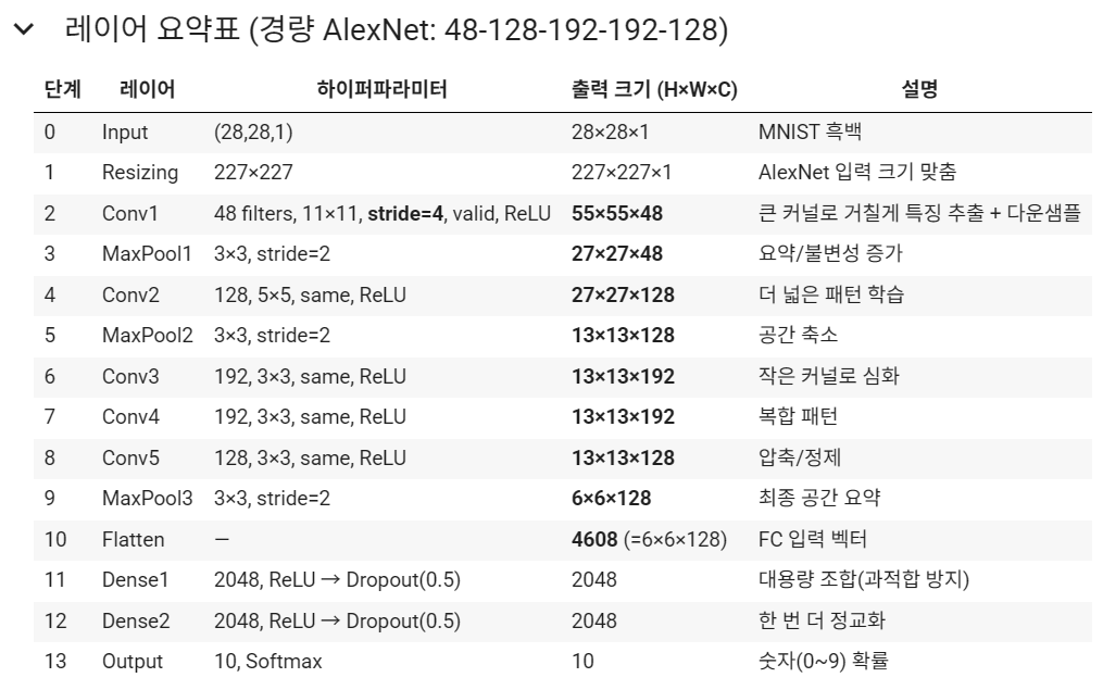
모델 아키텍처 정의

from tensorflow.keras.models import Sequential
from tensorflow.keras.layers import (
    Input, Resizing, Conv2D, MaxPooling2D, Flatten, Dense, Dropout
)

# 모델 아키텍처 정의
def build_alexnet_light_mnist(input_shape=(28,28,1), num_classes=10):
  model = Sequential([
      # 입력층
      Input(shape=(28,28,1)),
      Resizing(227,227),

      # 합성곱층 * 5
      Conv2D(filters = 48, kernel_size = 11, strides = 4, activation = 'relu'),
      MaxPooling2D(pool_size = 3, strides = 2),

      Conv2D(128, 5, padding = 'same', activation = 'relu'),
      MaxPooling2D(pool_size = 3, strides = 2),

      Conv2D(192, 3, padding = 'same', activation = 'relu'),
      Conv2D(192, 3, padding = 'same', activation = 'relu'),
      Conv2D(128, 3, padding = 'same', activation = 'relu'),
      MaxPooling2D(pool_size = 3, strides = 2),

      # 분배층
      Flatten(),
      Dense(512, activation = 'relu'),
      Dropout(0.5),
      Dense(512, activation = 'relu'),
      Dropout(0.5),

      # 출력층
      Dense(10, activation = 'softmax')
  ])
  
  return model

모델 확인

model = build_alexnet_light_mnist()
model.summary()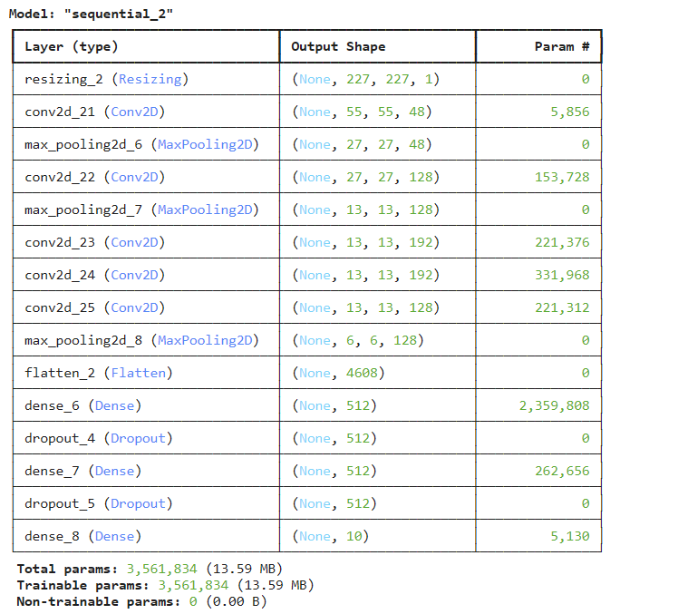

6. 모델 컴파일하기

model.compile()의 역할

케라스 모델을 학습하기 전에,

어떤 방식으로 최적화할지(optimizer)
손실(loss) 계산을 어떻게 할지
학습 성능을 어떤 지표(metrics)로 평가할지
를 미리 정해주는 단계이다.

6-1. 모델 컴파일

손실 함수, 옵티마이저, 메트릭 정의

model.compile(optimizer = 'adam',
              loss = tf.keras.losses.SparseCategoricalCrossentropy(from_logits=False),
              metrics = ['accuracy'],
  )

훈련 데이터를 이용해 모델 학습

model.fit(train_images, train_labels, epochs = 5)

epochs이 높을수록 성능이 좋아진다. 사용할 수 있는 GPU가 한정적인 관계로 굉장히 낮은 숫자인 5로 진행한다.

테스트 데이터로 모델 평가. 손실과 정확도 출력

test_loss, test_acc = model.evaluate(test_images, test_labels, verbose=2)

print('테스트 loss:', test_loss, '테스트 정확도:', test_acc)

결과:
313/313 - 4s - 14ms/step - accuracy: 0.9840 - loss: 0.0657
테스트 loss: 0.06571889668703079 테스트 정확도: 0.984000027179718

6-2. 예측 결과 시각화

predictions = model.predict(test_images)
num_rows = 3
num_cols = 3
num_images = num_rows * num_cols
plt.figure(figsize=(2*num_cols, 2*num_rows))
for i in range(num_images):
    plt.subplot(num_rows, num_cols, i+1)
    plt.imshow(test_images[i], cmap=plt.cm.binary)
    plt.xticks([])
    plt.yticks([])
    predicted_label = np.argmax(predictions[i])
    true_label = test_labels[i]
    if predicted_label == true_label:
        color = 'green'
    else:
        color = 'red'
    plt.xlabel("{} ({})".format(predicted_label, true_label), color=color)
plt.show()

7. VGGNet 한눈에 보기 (VGG-16 기준)

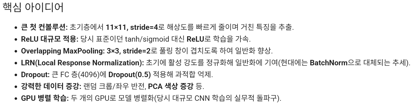
핵심 아이디어

작은 3×3 컨볼루션을 여러 번 쌓기: 큰 커널(예: 5×5) 한 번보다, 3×3 두 번이
- 파라미터가 더 적고(5×5=25 vs 3×3×2=18),
- 비선형성(ReLU)이 2번 들어가서 표현력이 높아짐.
단순하고 규칙적인 구조: 같은 크기의 Conv를 2~3번 반복 → MaxPool(2×2, s=2) 로 다운샘플.
깊이 증가: 블록을 내려갈수록 채널 수를 64→128→256→512→512로 증가.
분류기: Flatten → FC(4096) ×2 → Softmax.
원본 입력: 224×224×3 (ImageNet).

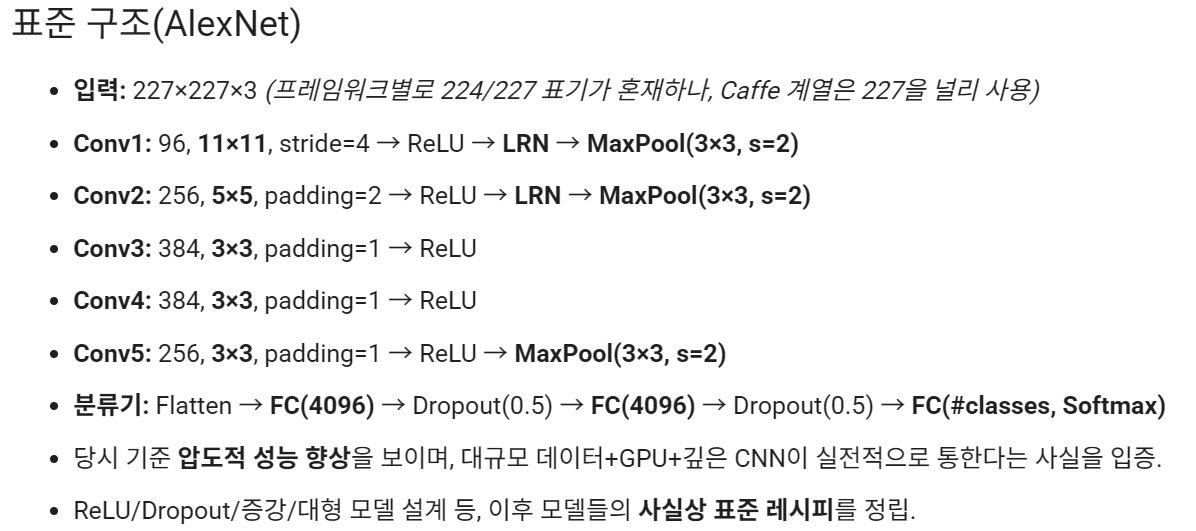
표준 구조(VGG-16)

Block1: [Conv(64) ×2] → MaxPool
Block2: [Conv(128) ×2] → MaxPool
Block3: [Conv(256) ×3] → MaxPool
Block4: [Conv(512) ×3] → MaxPool
Block5: [Conv(512) ×3] → MaxPool
Flatten → Dense(4096) → Dropout(0.5) → Dense(4096) → Dropout(0.5) → Dense(#classes, Softmax)

작은 필터를 깊게 쌓아 유효 수용영역을 키우면서, 파라미터를 절약하고 비선형 변환을 늘림.
규칙적인 패턴 덕에 구현·이해가 쉽고, 전이학습(backbone)으로도 많이 쓰임.

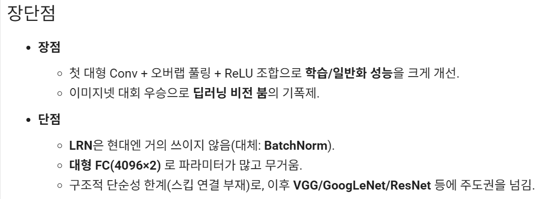
장단점

장점: 단순함, 재현 용이, 깊이에 따른 성능 향상.
단점: FC가 커서 파라미터 수가 매우 큼(VGG-16 전체 ~138M, 224×224×3 기준). 메모리/연산 무겁다.

실습 팁(MNIST)

MNIST(28×28×1)는 입력을 224×224로 리사이즈해 구조를 보존하여 실습 가능.
가벼운 실습용:
- FC 4096 → 512로 축소 또는 Flatten 대신 GlobalAveragePooling 사용.
- 채널 수를 절반으로 줄인 경량 VGG도 효과적.
원본 VGG에는 BatchNorm이 없음(후속 변형인 VGG-16-BN은 있음). 수렴 안정화용으로 BN을 추가 실험 가능.

7-1. 실습 진행

from tensorflow.keras.models import Sequential
from tensorflow.keras.layers import (
    Input, Resizing, Conv2D, MaxPooling2D, Flatten,
    Dense, Dropout, GlobalAveragePooling2D
)

# 경량 버전
def build_vgg16_mnist_light(input_shape=(28,28,1), num_classes=10):
    m = Sequential([
        Input(shape=input_shape),
        Resizing(224, 224),

        Conv2D(32, 3, padding='same', activation='relu'),
        Conv2D(32, 3, padding='same', activation='relu'),
        MaxPooling2D(2),

        Conv2D(64, 3, padding='same', activation='relu'),
        Conv2D(64, 3, padding='same', activation='relu'),
        MaxPooling2D(2),

        Conv2D(128, 3, padding='same', activation='relu'),
        Conv2D(128, 3, padding='same', activation='relu'),
        Conv2D(128, 3, padding='same', activation='relu'),
        MaxPooling2D(2),

        Conv2D(256, 3, padding='same', activation='relu'),
        Conv2D(256, 3, padding='same', activation='relu'),
        Conv2D(256, 3, padding='same', activation='relu'),
        MaxPooling2D(2),

        Conv2D(256, 3, padding='same', activation='relu'),
        Conv2D(256, 3, padding='same', activation='relu'),
        Conv2D(256, 3, padding='same', activation='relu'),
        MaxPooling2D(2),

        # Flatten 대신 GAP로 파라미터 크게 절감
        GlobalAveragePooling2D(),
        Dense(256, activation='relu'),
        Dropout(0.5),
        Dense(num_classes, activation='softmax'),
    ])
    return m

모델 확인

model = build_vgg16_mnist_light()
model.summary()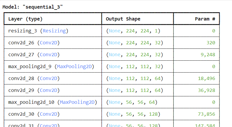

모델 컴파일. 손실 함수, 옵티마이저, 메트릭 정의

model.compile(optimizer='adam',
              loss=tf.keras.losses.SparseCategoricalCrossentropy(from_logits=False),
              metrics=['accuracy'])

훈련 데이터를 이용해 모델 학습

model.fit(train_images, train_labels, epochs=5)

테스트 데이터로 모델 평가. 손실과 정확도 출력

test_loss, test_acc = model.evaluate(test_images, test_labels, verbose=2)
print('테스트 loss:', test_loss, '테스트 정확도:', test_acc)

참고

#Keras/TensorFlow Applications로 제공되는 VGG16, VGG19

from keras.applications import VGG16, VGG19
from keras.applications.vgg16 import preprocess_input
from keras import layers, models
import tensorflow as tf

# MNIST 흑백 → RGB 3채널 + 224 리사이즈
inputs = layers.Input((28,28,1))
x = layers.Resizing(224, 224)(inputs)
x = tf.image.grayscale_to_rgb(x)  # (H,W,3)

# ① 사전학습 사용 + 내가 만든 분류기
base = VGG16(weights='imagenet', include_top=False, input_tensor=x)
base.trainable = False
x = layers.GlobalAveragePooling2D()(base.output)
outputs = layers.Dense(10, activation='softmax')(x)
model = models.Model(inputs, outputs)

짱아

짱아의 개발 일지

이전 포스트

딥러닝 회귀 모델 구현하기

다음 포스트

TensorFlow로 CNN 모델 구축

로봇영상처리를 위한 AI모델 학습

0. 환경설정

MNIST를 활용한 간단한 CNN 모델 만들기

1. MNIST 알아보기

필요 라이브러리 및 tensorflow 불러오기

Keras API를 활용해서 MNIST 불러오기

2. 데이터 확인해보기

train_images 데이터 확인

정답 데이터도 확인해보기

시각화해서 확인하기

3. 데이터 전처리 - 정규화하기

최소값과 최대값 확인하기

픽셀 값 범위를 [0, 255]에서 [0, 1]로 정규화

4. 모델 정의 - TensorFlow를 이용한 CNN 모델 만들기

4-1. filters 이해하기

3x3 필터 2개 사용, ReLU 활성화 적용 2D 합성곱층

2x2 필터 2개 사용, ReLU 활성화 적용 2D 합성곱층

4-2. kernel_size 이해하기

4-3. strides 이해하기

3x3 필터 2개 사용, 스텝사이즈 2, ReLU 활성화 적용 2D 합성곱층

3x3 필터 2개 사용, 스텝사이즈 2, ReLU 활성화 적용 2D 합성곱층

4-4. padding 이해하기

3x3 필터 2개 사용, 패딩 적용, ReLU 활성화 적용 2D 합성곱층

5. [미션 1] TensorFlow로 모델 architecture 직접 만들기

5-1. 기본 설명

5-2. AlexNet (레이어 구조)

5-3. 미션 시작

모델 아키텍처 정의

모델 확인

6. 모델 컴파일하기

model.compile()의 역할

6-1. 모델 컴파일

손실 함수, 옵티마이저, 메트릭 정의

훈련 데이터를 이용해 모델 학습

테스트 데이터로 모델 평가. 손실과 정확도 출력

6-2. 예측 결과 시각화

7. VGGNet 한눈에 보기 (VGG-16 기준)

핵심 아이디어

표준 구조(VGG-16)

장단점

실습 팁(MNIST)

7-1. 실습 진행

모델 확인

모델 컴파일. 손실 함수, 옵티마이저, 메트릭 정의

훈련 데이터를 이용해 모델 학습

테스트 데이터로 모델 평가. 손실과 정확도 출력

참고

딥러닝 회귀 모델 구현하기

Pytoch로 CNN모델 구축하기

0개의 댓글