제로베이스 6주차

터미널을 통해 jupyter notebook 실행하는 방법?

-> conda activate ds_study : ds_study 환경설정
-> cd Documents/ : 문서로 폴더 이동
-> cd ds_study : ds_study 폴더로 이동
-> jupyter notebook : 주피터 노트북 실행

4월3일 학습

년도별 데이터 컬럼 삭제

• del()
• drop()

인덱스 변경

• set_index() : 선택한 컬럼을 데이터 프레임의 인덱스로 지정

상관계수

• corr() : correlation의 약자, 상관계수가 0.2 이상인 데이터를 비교

4월4일 학습

matplotlib

• 파이썬의 대표 시각화 도구
• plt로 많이 naming하여 사용
• jupyter Notebook 유저의 경우 matplotlib의 결과가 out session에 나타나는 것이 유리하므로 %matplotlib inline 옵션을 사용한다.

예제1: 그래프 기초

삼각함수 그리기

• np.arange(a,b,s):a부터 b까지 s의 간격
• np.sin(value)

import numpy as np

t = np.arange(0, 12, 0.01)
y = np.sin(t)

plt.figure(figsize=(10,6))
plt.plot(t, np.sin(t))
plt.plot(t, np.cos(t))
plt.show()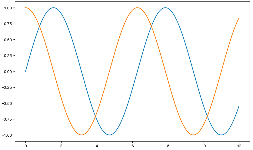

1. 격자무늬 추가
2. 그래프 제목 추가
3. x축, y축 제목 추가
4. 주황색, 파란색 선 데이터 의미 구분

def drawGraph(): 
    plt.figure(figsize=(10,6))
    plt.plot(t, np.sin(t), label="sin")
    plt.plot(t, np.cos(t), label="cos")
    plt.grid(True) #배경 격자 표시
    plt.legend(loc="lower left") 
# upper, lower, left, right  범례 위치 설정 가능
    plt.title("Example of sinewave")
    plt.xlabel("time")
    plt.ylabel("Amplitude")
    plt.show()
    
    drawGraph()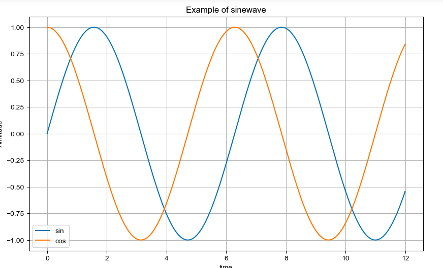

t = np.arange(0, 5, 0.5)
t

array([0. , 0.5, 1. , 1.5, 2. , 2.5, 3. , 3.5, 4. , 4.5])

plt.figure(figsize=(10,6))
plt.plot(t, t, "r--") #red---
plt.plot(t, t ** 2, "bs") #blue
plt.plot(t, t ** 3, "g^") #grin
plt.show()

#t = [0,1,2,3,4,5,6]
t = list(range(0,7))
y = [1,4,5,8,9,5,3]


def drawGraph():
    
    plt.figure(figsize=(10,6))

    plt.plot(
        t,
        y,
        color = "skyblue",
        linestyle = "dashed", #점선
        marker = ">",
        markerfacecolor="blue",
        markersize="10",)

    plt.xlim([-0.5,6.5])
    plt.ylim([0.5, 9.5])
    plt.show()

drawGraph()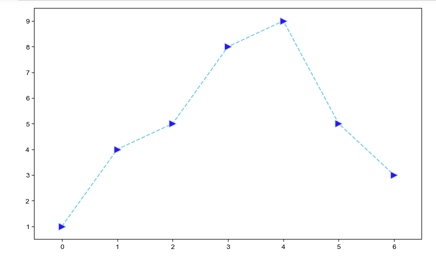

예제3 : scatter plot

t = np.array(range(0,10))
y = np.array([9, 8, 7, 9, 8, 3, 2, 4, 3, 4])

def drawGraph():
    plt.figure(figsize=(20,6))
    plt.scatter(t, y)
    plt.show()
    
drawGraph()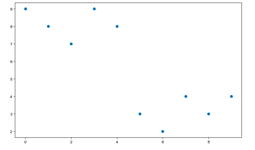

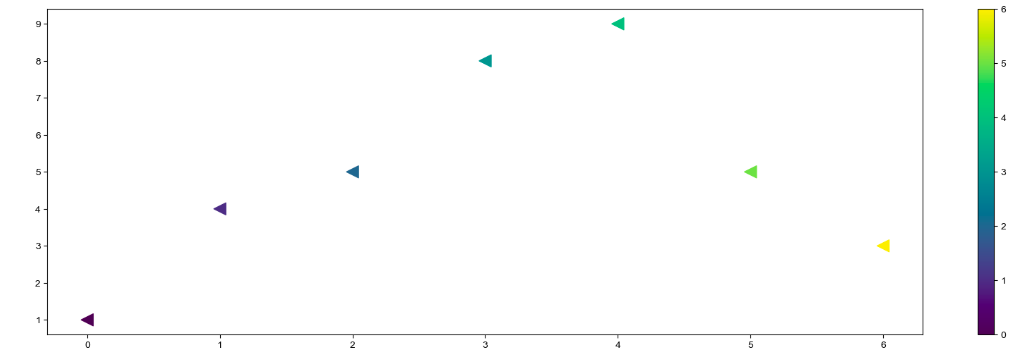
colormap = t

def drawGraph():
    plt.figure(figsize=(20, 6))
    plt.scatter(t, y, s=150 , c=colormap, marker="<")
    plt.colorbar()
    plt.show()
    
drawGraph()

4월5일 학습

Analysis Seoul Crime