[논문 리뷰] Diffuse to Detect: Generative Diffusion Models for Unsupervised IC Anomaly Detection (arXiv 2026)
Paper: Diffuse to Detect: Generative Diffusion Models for Unsupervised IC Anomaly Detection
Authors: Yuxuan Yin, Chen He, Todd Jacobs, Jialei He, Boxun Xu, Robert Jin, Peng Li
Affiliations: University of California Santa Barbara, NXP Semiconductors
Version: arXiv:2605.26468v1, May 26, 2026
Keywords: IC Testing, Latent Defect, Unsupervised Anomaly Detection, Diffusion Transformer, Semiconductor Manufacturing, Wafer Position Embedding
Part I. 연구 배경과 논문 개요
0. Functional Test를 통과한 불량은 어떻게 찾을까?
반도체 테스트의 기본 목적은 불량 die가 고객에게 전달되기 전에 걸러내는 것이다. 명확한 short, open, timing violation처럼 specification을 벗어나는 고장은 기존 functional test로 비교적 쉽게 제거할 수 있다. 더 어려운 문제는 현재의 functional criterion은 통과하지만 물리적 약점이 남아 있어 사용 중 고장으로 이어질 수 있는 latent defect다.
예를 들어 gate oxide의 약한 지점이나 작은 resistive short는 nominal condition에서 정상 동작할 수 있다. 그러나 leakage current, delay margin, voltage response처럼 수천 개의 parametric measurement를 함께 보면 정상 die와 미묘하게 다른 분포를 보일 수 있다. 자동차용 semiconductor에서 이러한 latent defect는 zero-defect quality 달성을 가로막고, high-performance computing에서는 Silent Data Corruption으로 이어질 수 있다.
문제는 latent defect가 극도로 희소하다는 것이다. 이 논문의 산업 데이터에서도 수천~수만 개 die 가운데 확인된 anomaly는 수 개에서 수십 개 수준이다. Label을 충분히 모아 supervised classifier를 학습하기 어렵고, 정상 die를 조금만 과도하게 제거해도 product yield가 크게 떨어진다.
이 논문은 다음 질문에서 출발한다.
정상 die만으로 diffusion model을 학습한 뒤, noise를 제대로 예측하지 못하는 die를 찾으면 label 없이도 latent defect를 선별할 수 있지 않을까?
저자들은 약 1,000~3,000개의 IC parametric feature를 128차원 latent로 압축하고, 이를 1D token sequence로 바꾼 뒤 Diffusion Transformer로 정상 분포를 학습한다. 여기에 wafer 내 die 좌표를 positional embedding으로 넣어 edge-center variation과 실제 anomaly를 구분하려 한다.
이 연구의 핵심은 diffusion으로 sample을 생성하는 것이 아니다. 중간 diffusion timestep에서 주입한 noise를 model이 얼마나 정확히 예측하는지를 anomaly score로 사용한다. Full reverse diffusion chain 없이 10회의 forward pass만 수행하기 때문에 wafer-scale screening에 적용할 수 있다는 주장이다.
그러나 결과를 자세히 보면 더 중요한 질문이 남는다.
- Dense MLP가 모든 원 feature를 섞은 뒤 만든 latent token에 정말 “test flow의 semantic order”가 남아 있는가?
- 95% yield에서 anomaly를 더 회수해도 정상 die 5%를 추가 폐기하는 비용은 감당 가능한가?
- 논문이 강조하는 feature localization은 실제 실험으로 검증됐는가, 아니면 future work인가?
이 리뷰에서는 성능 수치뿐 아니라 이 세 질문을 중심으로 논문을 읽어본다.
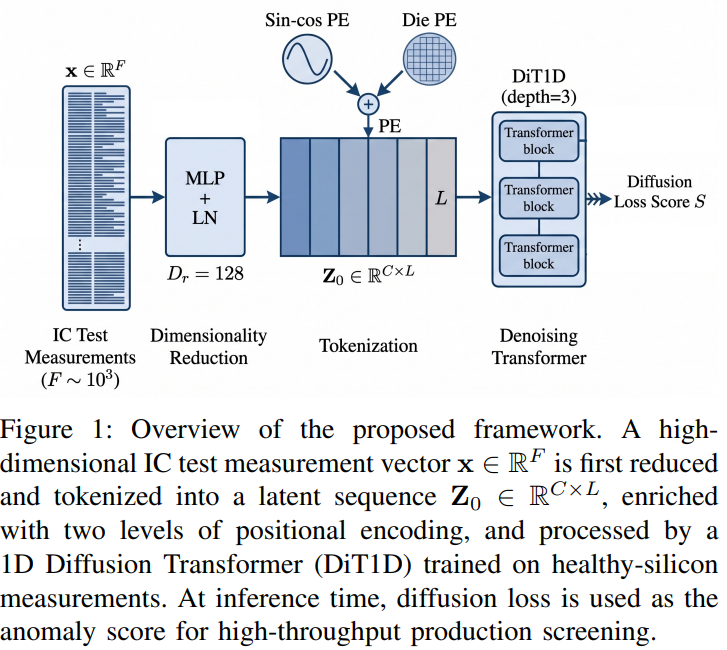
“고차원 parametric test measurement를 latent token sequence로 변환하고, 정상 die로 학습한 1D Diffusion Transformer의 noise-prediction error를 anomaly score로 사용한다.”
1. Abstract 요약
Latent defect screening은 세 가지 이유로 어렵다.
- Failure rate가 극도로 낮다.
- 한 die마다 수천 개 test feature가 생성된다.
- Labelled anomaly가 거의 없다.
저자들은 고차원 IC test data를 위한 완전 비지도 anomaly detection framework인 Diffuse to Detect를 제안한다. Raw measurement는 MLP autoencoder를 통해 낮은 차원으로 압축되고, 구조화된 token sequence로 reshape된다. Token 위치를 나타내는 sinusoidal embedding과 wafer 위 die 위치를 나타내는 per-device embedding이 더해진다.
이 latent sequence에 Gaussian noise를 주입한 뒤 1D Diffusion Transformer(DiT1D)가 noise를 예측하도록 정상 die만으로 학습한다. Test die가 정상 분포에 속하면 noise를 비교적 잘 예측하지만, distribution 밖의 anomaly에서는 prediction error가 커진다. 저자들은 여러 중간 diffusion timestep의 noise-prediction loss를 평균해 anomaly score를 만든다.
16 nm automotive IC의 두 release dataset에서 DiT1D는 classical, deep learning, diffusion baseline보다 높은 AUROC와 yield-constrained recall을 보인다. 또한 reverse diffusion reconstruction residual을 이용하면 어떤 measurement 또는 test program이 정상에서 벗어났는지 분석할 수 있다고 제안한다.
Abstract를 한 문장으로 압축하면
수천 개 IC test measurement를 작은 token sequence로 압축하고 wafer 위치를 조건으로 넣은 Diffusion Transformer가 정상 latent distribution의 noise를 학습하게 하면, noise-prediction error만으로 극희소 latent defect를 선별할 수 있다.
먼저 구분해야 할 두 가지
- 학습에 anomaly label을 loss로 사용하지 않는다는 의미에서 unsupervised다. 그러나 anomaly를 training에서 제외하기 위해 health label을 사용하고, evaluation에도 confirmed anomaly label을 사용한다.
- Main screening score는 reconstruction error가 아니라 noise-prediction error다. Feature-level reconstruction residual은 conclusion에서 제안하는 후속 분석 방식이며 본 실험에서 localization accuracy가 검증되지는 않았다.
2. 전체 논문 총 정리
| 항목 | 내용 |
|---|---|
| 연구 목표 | Functional test를 통과한 latent defect의 비지도 선별 |
| 데이터 | 16 nm automotive chip product의 두 release version |
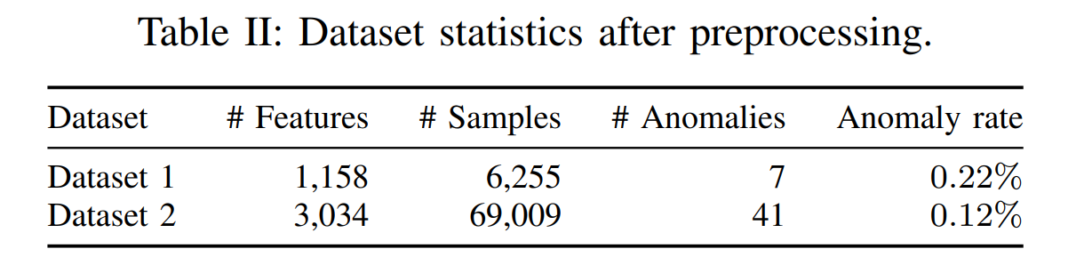
| Dataset 1 | 1,158 features, 6,255 samples, 7 anomalies |
| Dataset 2 | 3,034 features, 69,009 samples, Table II 기준 41 anomalies |
| Train data | Label-normal device의 50% |
| Test data | 나머지 normal 50% + 모든 anomaly |
| Input processing | Feature selection, missing-value filtering, within-wafer z-score |
| Latent representation | 차원 → MLP encoder → |
| Tokenization | , latent sequence |
| Position information | Latent token sin-cos PE + die gated MLP PE |
| Denoiser | 3-block 1D Diffusion Transformer, hidden 256, 4 heads |
| Diffusion | 1,000 steps, cosine schedule |
| Inference score | 의 noise-prediction MSE 평균 |
| Forward passes/device | 10회 |
| Primary metrics | AUROC, AUCPR, Recalled@95% Yield |
| Dataset 1 result | 0.771 / 0.0250 / 3 |
| Dataset 2 result | 0.639 / 0.0023 / 7 |
| 핵심 ablation | Die PE, autoencoder, transformer backbone 모두 기여 |
Part II. 문제 정의와 핵심 아이디어
3. Step 01 - Problem: 기존 연구의 결정적 결함은 무엇인가?
3.1 Latent defect는 supervised learning을 적용하기 어려울 만큼 희소하다
Mature semiconductor process에서 latent failure rate는 ppm(parts per million) 단위까지 내려간다. 이 논문의 작은 dataset에서도 anomaly는 7개뿐이다. 이런 환경에서는 다음 문제가 생긴다.
- Classifier가 majority normal class로 collapse하기 쉽다.
- Train/validation split마다 anomaly 수가 크게 달라진다.
- 새로운 failure mechanism은 과거 label로 정의되지 않는다.
- Failure analysis를 통해 확정 label을 얻는 데 시간과 비용이 든다.
따라서 “모든 불량 유형을 미리 학습한다”는 closed-set classification보다 정상 die의 distribution을 학습하고 벗어나는 sample을 찾는 one-class 접근이 자연스럽다.
3.2 IC parametric test는 고차원이며 의미가 이질적이다
현대 production test는 한 die에서 수천 개 measurement를 만든다.
- leakage current
- propagation delay
- voltage margin
- stress response
- application-specific parametric result
각 feature는 scale과 물리적 의미가 다르고, feature 수가 sample의 유효 자유도보다 훨씬 크다. Raw space의 Euclidean distance나 density estimation은 curse of dimensionality에 취약하다.
3.3 Wafer 위치 변화가 anomaly처럼 보일 수 있다
Wafer center와 edge에서는 systematic process variation 때문에 정상 die의 measurement distribution도 다를 수 있다. Die coordinate를 무시하면 정상적인 edge-center shift가 outlier score를 키운다.
즉, anomaly detector는 다음을 구분해야 한다.
정상적인 wafer spatial variation
            vs.
개별 die의 비정상 parametric deviation
3.4 제조 현장에서는 false positive도 매우 비싸다
Defect를 놓치면 field return, warranty, safety risk가 발생한다. 반대로 정상 die를 anomaly로 잘못 제거하면 수율과 매출이 떨어진다. 따라서 단순 AUROC만 높이는 것으로는 부족하다.
필요한 질문은 다음과 같다.
- 정상 die를 99.9% 이상 통과시키면서 anomaly를 몇 개 잡는가?
- 추가 screening 또는 failure analysis가 필요한 die 수는 몇 개인가?
- 제품 가격과 defect escape cost를 함께 고려한 최적 threshold는 무엇인가?
3.5 기존 방법은 feature engineering 또는 modality mismatch에 의존한다
- SPC/PCA: domain expert가 중요한 feature와 threshold를 정해야 한다.
- Isolation Forest/OCSVM: 고차원 raw feature에서 불안정할 수 있다.
- Autoencoder: joint dependency를 충분히 표현하지 못하거나 anomaly까지 잘 복원할 수 있다.
- Image diffusion: 2D spatial patch라는 inductive bias가 tabular IC measurement에는 맞지 않는다.
- TabDDPM: feature vector를 flat unordered table로 처리해 test program structure를 활용하지 않는다.
핵심 연구 공백
Labelled defect와 수작업 feature engineering 없이, 수천 차원의 IC test measurement와 wafer 위치 효과를 동시에 학습하고, 극심한 class imbalance에서도 yield를 통제하며 latent defect를 선별할 방법이 부족하다.
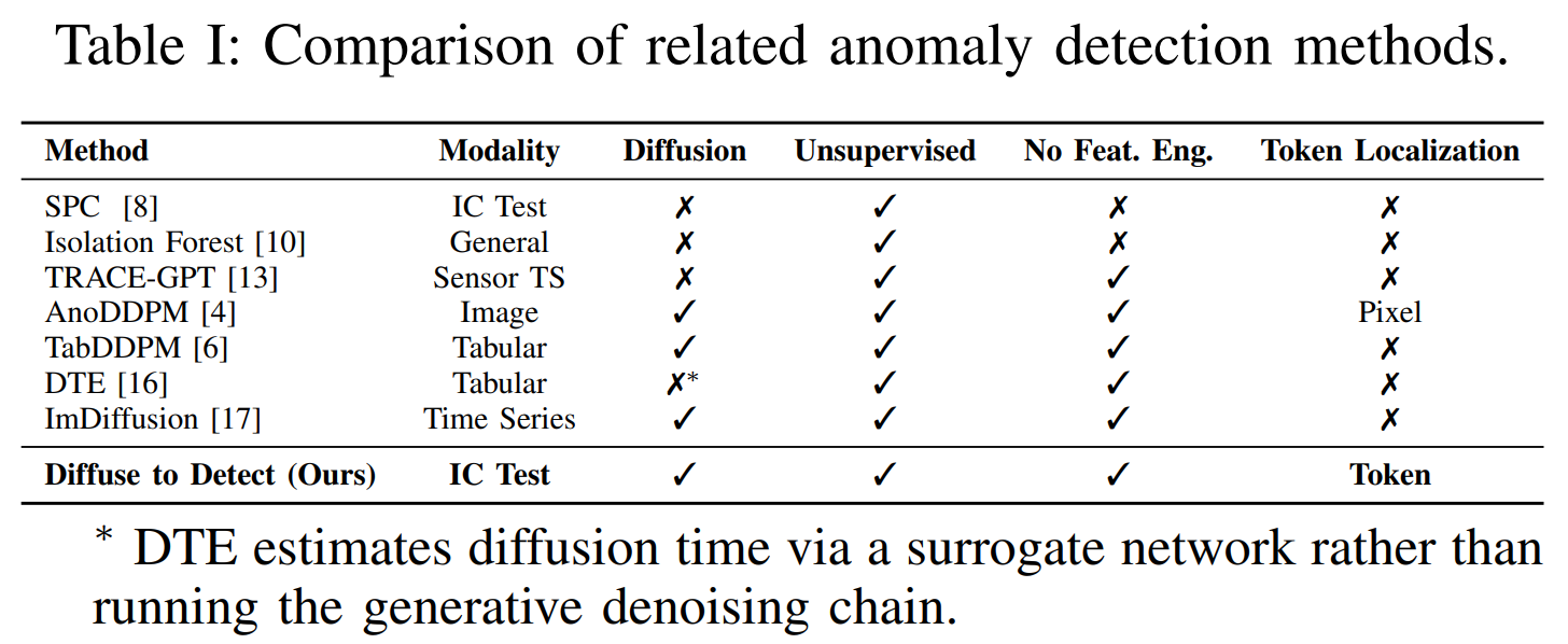
4. Related Work: 왜 SPC도, TabDDPM도 충분하지 않은가?
4.1 IC anomaly detection
| 방법 | 장점 | 한계 |
|---|---|---|
| SPC·Control chart | 가볍고 공정 엔지니어가 해석하기 쉬움 | Feature·threshold를 수작업으로 정의 |
| PCA | Dimension reduction과 residual score가 단순 | Nonlinear dependency 표현이 제한적 |
| Isolation Forest·OCSVM | Label 없이 적용 가능 | 수천 차원에서 distance/density가 불안정 |
| Autoencoder·VAE | Nonlinear normal representation 학습 | Anomaly reconstruction과 threshold 문제가 있음 |
| TRACE-GPT | Semiconductor sensor sequence를 generative model로 처리 | 장비 시계열 대상이며 IC tabular output과 다름 |
| Wafer bin map diffusion | Spatial defect pattern을 image로 탐지 | Binary pass/fail map이며 continuous parametric test와 다름 |
4.2 Diffusion anomaly detection
DDPM은 정상 data에 점진적으로 Gaussian noise를 넣고 이를 되돌리는 denoiser를 학습한다. 정상 sample은 학습 distribution 위에 있으므로 denoise하기 쉽고, anomaly는 denoising 또는 noise prediction error가 커진다는 논리다.
AnoDDPM, DiffusionAD와 같은 기존 연구는 주로 medical 또는 industrial image를 다룬다. Image에서는 spatial locality와 patch 구조가 자연스럽지만 IC test vector는 feature dimension 사이 거리가 물리적 인접성을 의미하지 않는다.
TabDDPM은 tabular diffusion의 대표 baseline이지만 flat vector에 ResNet-style MLP를 적용한다. 저자들은 이것이 feature 사이의 compound correlation과 test flow order를 충분히 활용하지 못한다고 본다.
4.3 Diffusion Transformer
DiT는 기존 DDPM의 U-Net denoiser를 Transformer로 바꾼 architecture다. Transformer는 다음 두 특성 때문에 이 논문의 문제에 적합하다고 주장된다.
- Variable-length token sequence와 positional encoding을 자연스럽게 처리
- Token별 output을 제공해 local residual 분석 가능
저자들은 2D image patch 대신 1D latent patch를 사용해 DiT를 IC test data에 맞춘다.
5. Step 02 - Idea: 이 논문만의 독창적인 한 줄 논리
IC test vector를 그대로 diffusion하지 말고, wafer 위치가 반영된 짧은 latent token sequence로 압축한 뒤 Transformer가 정상 token의 noise를 예측하게 하면, prediction error로 latent defect를 빠르게 선별할 수 있다.
전체 pipeline은 다음과 같다.
IC parametric measurements x ∈ R^F
             ↓
Within-wafer normalization
             ↓
MLP Autoencoder: F → 128
             ↓
Reshape: 4 channels × 32 positions
             ↓
Feature-position sin-cos PE
       + Die-coordinate gated PE
             ↓
Gaussian forward diffusion at 10 mid-range timesteps
             ↓
1D Diffusion Transformer predicts ε
             ↓
Average noise-prediction MSE
             ↓
Anomaly score and yield-constrained ranking
왜 reconstruction chain을 끝까지 돌리지 않는가?
일반적인 diffusion reconstruction은 수백~수천 번의 reverse step이 필요하다. 모든 die를 production scale로 평가하기에는 비싸다. 이 논문은 이미 알고 있는 noise 을 model이 얼마나 잘 맞히는지만 본다.
Known noise ε
   ↓ add to latent
Noisy latent Z_t
   ↓ DiT1D
Predicted noise ε_θ
   ↓
||ε - ε_θ||² = anomaly evidence
따라서 inference는 생성이 아니라 normal-distribution compatibility test에 가깝다.
Part III. 데이터와 제안 방법론
6. Dataset: 16 nm Automotive IC의 실제 Parametric Test
데이터는 16 nm automotive chip product의 두 release version에서 수집됐다. 한 row는 (lot, wafer, die) 단위의 test outcome이며 다음 정보를 포함한다.
- binary health label
lot_key,wf_keydie_x,die_y- 다수의 continuous parametric measurements
| Dataset | Features | Total samples | Table II anomalies | 표기 anomaly rate |
|---|---|---|---|---|
| Dataset 1 | 1,158 | 6,255 | 7 | 0.22% |
| Dataset 2 | 3,034 | 69,009 | 41 | 0.12% |
Anomaly rate 숫자를 읽을 때 주의할 점
7/6,255는 약 0.11%이고 41/69,009는 약 0.06%이므로 Table II의 0.22%와 0.12%와 직접 일치하지 않는다. 정상 die 절반만 test에 넣고 모든 anomaly를 test에 넣는 protocol을 적용하면 다음처럼 거의 일치한다.
- Dataset 1:
- Dataset 2:
따라서 표의 # Samples는 전체 data, Anomaly rate는 test split prevalence로 계산된 것으로 추정된다. 논문이 이를 명시적으로 구분하지 않아 처음 읽을 때 혼동하기 쉽다.
6.1 Feature selection과 missing value 처리
저자들은 정규식으로 task-specific parametric measurement column을 선택한다. Missing ratio가 threshold보다 큰 column은 제거하고, 남은 feature 중 missing value가 하나라도 있는 device row는 삭제한다.
“Manual feature engineering이 없다”는 주장은 handcrafted statistical feature를 만들지 않는다는 뜻이지, preprocessing이나 feature selection이 전혀 없다는 뜻은 아니다.
6.2 Within-wafer z-score
각 (lot_key, wf_key) group 안에서 feature별 mean과 standard deviation을 계산한다.
이는 lot·wafer-level offset을 줄여 개별 die deviation에 집중하게 한다. Die coordinate는 normalization vector에 넣지 않고 raw grid 값으로 positional embedding에만 사용한다.
다만 이 normalization에는 두 가지 deployment 조건이 따른다. 첫째, 한 die를 검사하는 순간 독립적으로 score를 계산하려면 해당 wafer의 mean·standard deviation이 아직 완성되지 않았을 수 있으므로, 충분한 die가 누적되거나 wafer test가 끝날 때까지 기다려야 한다. 둘째, train/test를 나눈 뒤에도 같은 wafer 전체의 통계를 함께 사용했다면 test distribution이 preprocessing에 들어가는 transductive leakage가 된다. 논문은 group statistic을 split 전·후 어느 단계에서 계산했는지 명확히 밝히지 않는다.
Normalization 설명 자체에도 재현성상 모호함이 있다. Methodology의 Eq. (1) 주변에서는 D_train 통계로 모든 feature를 zero mean·unit variance로 표준화한다고 쓰지만, Experiment section에서는 global standardization 대신 within-wafer z-score를 사용한다고 설명한다. 두 normalization을 순차 적용했는지 within-wafer 방식만 사용했는지 명확히 할 필요가 있다.
6.3 Train-test split
- Label-normal die의 50%: training
- 나머지 normal die 50%: test
- 모든 anomaly: test
- Fixed random seed: 42
Model loss에는 anomaly label을 사용하지 않지만, clean normal training set을 만들기 위해 health label을 사용한다. 따라서 “label-free deployment”를 주장하려면 anomaly가 일부 섞인 training data에서도 안정적인지 contamination test가 필요하다.
7. Proposed Method 1 - Autoencoder로 3,000차원을 128차원으로 압축한다
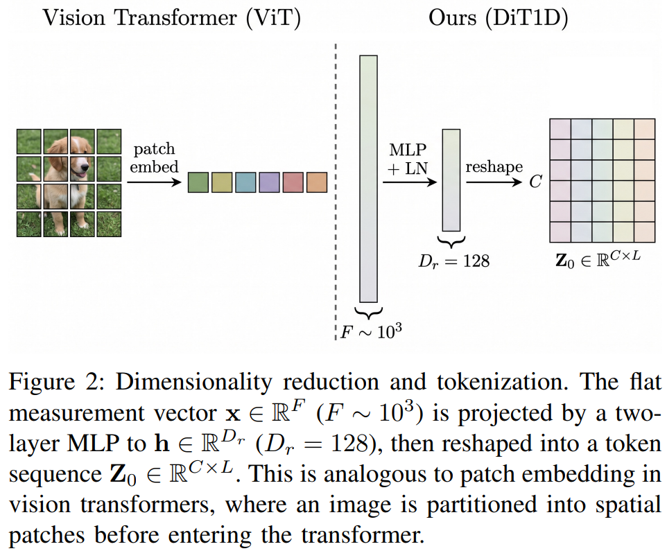
Raw feature vector 를 바로 Transformer에 넣으면 계산량이 크고 statistical conditioning이 나쁘다. 저자들은 2-layer MLP encoder로 128차원 representation을 만든다.
LayerNorm은 latent의 scale을 안정화해 Gaussian diffusion을 쉽게 만든다.
학습은 두 단계다.
-
Autoencoder pretraining 50 epochs
Encoder와 symmetric decoder를 reconstruction MSE로 학습한다. -
Diffusion training 200 epochs
Encoder를 freeze하고 DiT1D만 noise-prediction loss로 학습한다.
Decoder는 main screening inference에는 사용되지 않는다. 원 measurement space의 feature residual을 계산하는 root-cause analysis에서만 필요하다.
Autoencoder가 필요한 이유
- 1,000~3,000개 feature를 128개 degree로 압축
- Raw-space diffusion의 optimization 불안정성 완화
- Transformer sequence 길이와 계산량 제어
- Noise가 많은 feature dimension의 redundancy 제거
그러나 reconstruction objective가 anomaly detection에 최적인 representation을 보장하는 것은 아니다. Joint training이나 self-supervised objective와의 비교는 수행하지 않았다.
8. Proposed Method 2 - 128차원 latent를 1D token으로 바꾼다
Encoder output 을 다음처럼 reshape한다.
기본 설정은 다음과 같다.
즉, 4차원 channel을 가진 32개 latent position을 만든다. 이후 Conv1d patch embedding의 patch size를 로 두어 16개 transformer token으로 만든다.
ViT patch와 정말 같은가?
저자들은 이를 image patch embedding과 유사하다고 설명한다. 하지만 중요한 차이가 있다.
- ViT patch는 원 image의 공간적으로 인접한 pixel을 보존한다.
- 이 논문의 token은 dense MLP가 모든 input feature를 섞어 만든 128개 latent dimension을 임의 순서로 reshape한 것이다.
따라서 latent position 1과 2가 같은 test program의 인접 measurement라는 보장은 없다. Transformer가 latent dependency를 학습할 수는 있지만, token 순서가 곧 “test flow의 semantic ordering”이라고 단정하기는 어렵다.
이 문제를 더 강하게 해결하려면 처음부터 test program별 feature block을 token으로 만들거나, group-wise encoder로 program identity를 보존해야 한다.
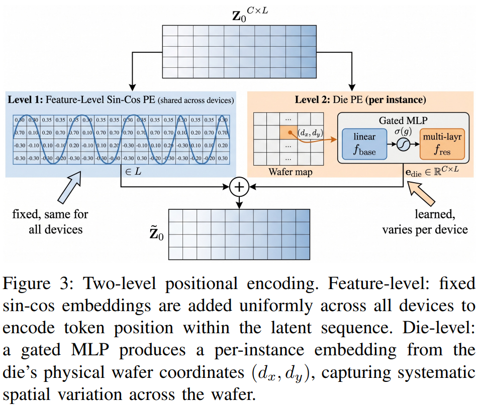
9. Proposed Method 3 - 두 종류의 Positional Encoding
논문은 token structure와 wafer geometry를 동시에 반영하기 위해 두 positional encoding을 사용한다.
9.1 Level 1: Feature-level sinusoidal PE
32개 latent position에 fixed sin-cos embedding을 더한다.
이 embedding은 모든 device에 동일하며 latent token의 순서를 구분한다.
9.2 Level 2: Per-device die positional embedding
Wafer 좌표 와 좌표별 sin-cos feature를 결합한다.
Gated MLP가 이를 shape의 embedding으로 변환한다.
Gate 는 0으로 initialize된다. 처음에는 좌표의 linear effect만 사용하고, 학습이 진행되면서 nonlinear residual이 점진적으로 활성화된다.
왜 die PE가 중요한가?
Wafer edge의 정상 die는 center die와 measurement distribution이 다를 수 있다. 좌표 조건이 없으면 model이 정상 spatial variation을 anomaly로 오해할 수 있다. Ablation에서도 die PE를 제거했을 때 AUROC가 0.234나 감소해 가장 큰 영향이 나타난다.
10. Proposed Method 4 - Latent Token 위의 Forward Diffusion
Clean latent 에 step의 Gaussian diffusion을 정의한다.
누적 noise schedule 를 사용하면 임의 timestep의 noisy latent를 한 번에 만들 수 있다.
Noise schedule은 cosine schedule이다.
Training objective는 standard DDPM simplified loss다.
정상 die만 학습했기 때문에 normal latent에서는 noise를 잘 예측하고, anomaly latent에서는 error가 커질 것이라는 가정이다.
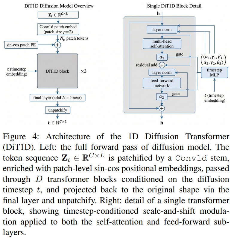
11. Proposed Method 5 - 1D Diffusion Transformer
11.1 1D patch embedding
를 Conv1d stem으로 patchify한다. 기본 patch size 이므로 16개 token이 만들어지고 hidden dimension 256으로 projection된다.
11.2 Timestep-conditioned Transformer block
각 block은 multi-head self-attention과 feed-forward network로 구성되며, diffusion timestep embedding이 adaptive LayerNorm의 scale·shift·gate를 제어한다.
기본 architecture는 다음과 같다.
| 구성 | 값 |
|---|---|
| Transformer blocks | 3 |
| Hidden dimension | 256 |
| Attention heads | 4 |
| Patch size | 2 |
| Input tokens | 16 |
| Total model parameters | 약 4M, decoder 포함 |
Final layer는 token을 다시 latent shape로 unpatchify하고 noise 을 출력한다.
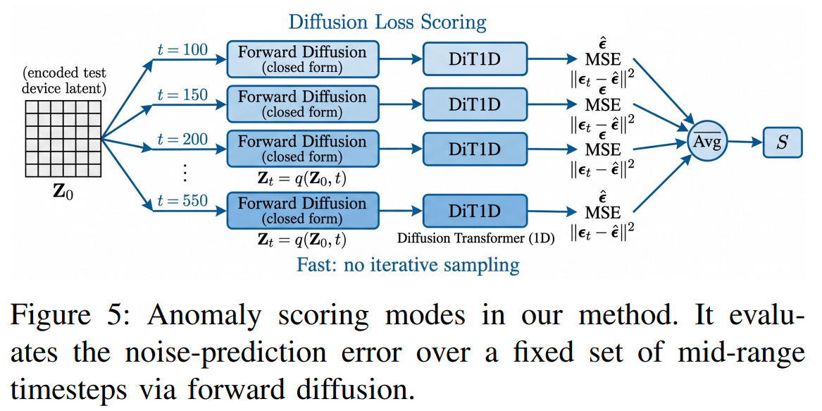
12. Anomaly Scoring: 1,000-step 생성 없이 10번만 평가한다
Inference에서는 다음 10개 timestep을 사용한다.
각 timestep에서 test latent에 noise를 한 번에 주입하고 DiT1D가 예측한 noise와 실제 noise의 MSE를 계산한다.
왜 mid-range timestep인가?
- 너무 작은 : input이 거의 clean해 noise prediction이 anomaly structure를 충분히 드러내지 못할 수 있다.
- 너무 큰 : 원 input 정보가 대부분 사라져 normal과 anomaly 구분이 약해질 수 있다.
- 중간 : input structure와 denoising difficulty가 함께 남는다.
다만 논문은 100~550을 사용한 이유를 직관적으로 설명할 뿐, timestep range나 forward-pass 수에 대한 ablation은 제공하지 않는다.
장점
- 1,000-step reverse sampling 불필요
- Device당 10회 independent forward pass
- Batch processing 가능
- Anomaly score가 단순한 scalar MSE
남은 문제
- Gaussian noise sample에 따라 score가 달라질 수 있다.
- Noise seed 반복에 대한 variance가 보고되지 않았다.
- A100에서 실제 device/s, latency, memory를 측정하지 않았다.
Part IV. 평가 방법과 실험 결과
13. Evaluation: AUROC만으로는 극희소 결함을 평가할 수 없다
13.1 AUROC
Random anomaly 하나가 random normal보다 높은 score를 받을 확률을 측정한다. 전체 ranking은 볼 수 있지만 class imbalance가 심하면 실제 top-ranked precision이 낮아도 높게 나올 수 있다.
13.2 AUCPR
Precision-recall curve 아래 면적으로 rare anomaly retrieval에 더 적합하다. Random classifier의 기대 AUCPR은 anomaly prevalence와 같다.
- Dataset 1 random level: 약 0.0022
- Dataset 2 random level: 약 0.0012
13.3 Recalled@95% Yield
정상 test die의 95%가 통과하도록 threshold를 설정한다. 즉, normal의 5%는 추가 screening 또는 reject 대상이 된다. 그 threshold 위에 놓인 confirmed anomaly 수를 Recalled로 보고한다.
이 metric은 다음 trade-off를 직접 반영하려는 시도다.
Threshold 완화 → anomaly recall 증가 / normal overkill 증가
Threshold 강화 → yield 증가 / defect escape 증가
그러나 95% yield는 mature automotive product에 매우 느슨할 수 있다. 실제 생산에서는 99%, 99.9%, 99.99%와 같은 더 높은 normal pass rate에서도 평가해야 한다.
14. Experimental Setup과 Baseline
14.1 Training
| 항목 | 설정 |
|---|---|
| Autoencoder pretraining | 50 epochs |
| Diffusion training | 200 epochs |
| Diffusion steps | 1,000 |
| Optimizer | AdamW |
| Learning rate | |
| Weight decay | |
| Batch size | 2,048 |
| Random seed | 42 |
| GPU | NVIDIA A100 80GB ×1 |
14.2 Baselines
총 20개가 넘는 unsupervised baseline과 비교한다.
| Category | Methods |
|---|---|
| Classical | IForest, OCSVM, COPOD, ECOD, FeatureBagging, HBOS, KNN, LODA, LOF, MCD, PCA |
| Deep learning | DAGMM, DROCC, GOAD, ICL, PlanarFlow, GANomaly, SLAD, DIF |
| Diffusion | TabDDPM, DTE-IG, DTE-C |
Baseline은 PyOD, official code, published default hyperparameter를 사용한다. 비교 범위는 넓지만, 제안 model은 Dataset 1의 depth와 patch size를 상세히 선택한 반면 baseline은 default 설정이므로 hyperparameter tuning budget이 동일하지 않을 가능성이 있다.
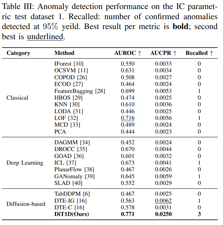
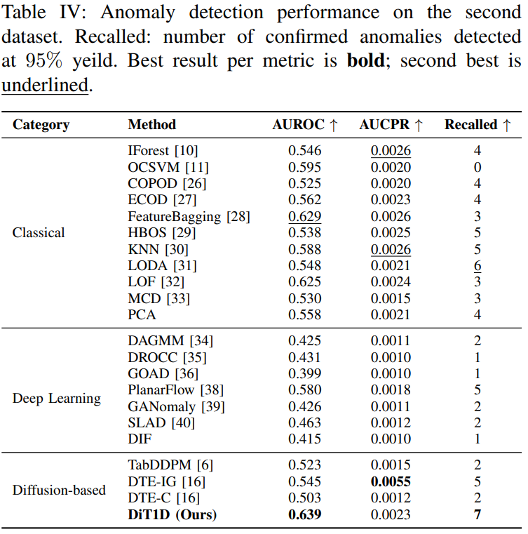
15. Results 1 - Dataset 1: Diffusion Transformer가 가장 분명하게 우세하다
Dataset 1의 핵심 결과는 다음과 같다.
| Method | AUROC | AUCPR | Recalled@95% Yield |
|---|---|---|---|
| LOF | 0.716 | 0.0056 | 1 |
| DTE-IG | 0.563 | 0.0062 | 1 |
| GANomaly | 0.645 | 0.0059 | 1 |
| DiT1D | 0.771 | 0.0250 | 3 |
15.1 AUROC
DiT1D의 0.771은 second-best LOF 0.716보다 0.055 높다. 완벽한 분리는 아니지만 다른 baseline보다 anomaly-normal ranking이 일관되게 좋다.
15.2 AUCPR
0.0250은 절대값으로는 2.5%지만 random level 0.22%보다 약 11배 높다. Second-best DTE-IG 0.0062보다 약 4배 높다. 극희소 anomaly에서 상대적 lift는 의미가 있다.
15.3 Recalled@95% Yield
7개 anomaly 중 3개를 회수한다. 다른 모든 baseline은 최대 1개만 회수한다. 즉, 5% normal overkill을 허용했을 때 defect recall은 다음과 같다.
Yield 관점의 절대적 해석
Dataset 1 test에는 대략 3,124개의 normal die가 있다. 95% yield threshold는 약 156개의 normal die를 추가로 screen out한다. 여기에 anomaly 3개를 잡는다고 단순 계산하면 threshold 위 candidate의 precision은 약 1.9% 수준이다.
이는 random ranking보다는 크게 좋지만, production에서 156개 good die를 희생해 3개 latent defect를 잡는 것이 경제적인지는 제품 가격과 field-failure cost를 함께 계산해야 한다.
16. Results 2 - Dataset 2: AUROC와 Yield Recall은 최고지만 AUCPR은 아니다
Dataset 2의 주요 결과는 다음과 같다.
| Method | AUROC | AUCPR | Recalled@95% Yield |
|---|---|---|---|
| IForest | 0.546 | 0.0026 | 4 |
| LODA | 0.548 | 0.0021 | 6 |
| HBOS | 0.538 | 0.0025 | 5 |
| KNN | 0.588 | 0.0026 | 5 |
| LOF | 0.625 | 0.0024 | 3 |
| DTE-IG | 0.545 | 0.0055 | 5 |
| DiT1D | 0.639 | 0.0023 | 7 |
16.1 무엇이 최고인가?
- AUROC: DiT1D 0.639로 최고
- Recalled@95% Yield: DiT1D 7로 최고
- AUCPR: DTE-IG 0.0055가 최고, DiT1D는 0.0023
따라서 Dataset 2에서는 DiT1D가 모든 metric의 SOTA라고 말할 수 없다. Production operating point인 95% yield에서 가장 많은 anomaly를 회수하고 전체 ranking도 가장 좋지만, precision-recall curve 전체에서는 DTE-IG가 더 우수하다.
DiT1D AUCPR 0.0023은 random level 0.0012의 약 1.9배에 불과하고, 일부 classical method의 0.0026보다도 낮다. Dataset 1의 강한 AUCPR 개선이 Dataset 2에서 그대로 재현되지는 않았다.
16.2 논문 내부의 anomaly 수 불일치
Table II는 Dataset 2에 anomaly가 41개라고 적는다. Train-test protocol은 모든 anomaly를 test에 넣는다고 설명한다. 그러나 Main Results 본문은 “test split에 존재하는 7개 anomaly를 모두 recall했다”고 서술한다.
가능한 해석은 다음 두 가지다.
- 41개 label anomaly 중 7개만 failure analysis로 confirmed되었다.
- Table II 또는 본문의 anomaly 수 표기가 잘못되었다.
논문은 이를 명확히 설명하지 않는다. Table IV의 Recalled=7이 41개 중 7개라면 recall은 17.1%이고, 실제 anomaly가 7개라면 recall은 100%다. 두 해석의 차이가 매우 크므로 최종 publication에서는 반드시 수정돼야 한다.
16.3 95% yield의 실제 candidate 수
Dataset 2 test normal은 약 34,484개로 추정된다. 정상 5%를 screen out하면 약 1,724개 good die가 candidate에 포함된다. 7개 anomaly를 회수해도 단순 precision은 약 0.4%다. High-volume production에서는 더 높은 yield operating point의 결과가 필요하다.
17. Results 3 - Ablation: 어떤 component가 실제로 중요한가?
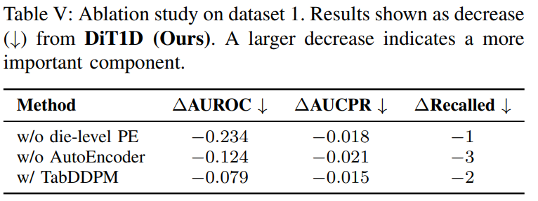
Table V는 Dataset 1에서 full DiT1D 대비 성능 감소를 보고한다. 이를 실제 score로 복원하면 다음과 같다.
| Variant | AUROC | AUCPR | Recalled |
|---|---|---|---|
| Full DiT1D | 0.771 | 0.025 | 3 |
| w/o die-level PE | 0.537 | 0.007 | 2 |
| w/o Autoencoder | 0.647 | 0.004 | 0 |
| TabDDPM-style MLP denoiser | 0.692 | 0.010 | 1 |
17.1 Die positional embedding
Die PE 제거 시 AUROC가 0.234 감소한다. 세 ablation 중 AUROC 하락이 가장 크다. Wafer location이 정상 variation의 강한 confounder라는 뜻이다.
하지만 이 결과는 두 방향으로 해석해야 한다.
- 긍정적: 위치 조건이 edge-center variation을 정상으로 설명한다.
- 주의: Random die split에서 같은 wafer의 다른 die가 train/test에 함께 있으면 spatial pattern을 쉽게 학습했을 수 있다.
새로운 lot·wafer에서 generalization하는지는 wafer-level split으로 검증해야 한다.
17.2 Autoencoder
Autoencoder를 제거하고 raw feature에서 diffusion하면 AUCPR이 0.021 감소하고 Recalled가 3에서 0이 된다. 고차원 raw diffusion보다 compact latent diffusion이 훨씬 안정적이라는 가장 강한 근거다.
17.3 Transformer vs. MLP denoiser
같은 latent encoder를 유지하고 DiT1D를 TabDDPM-style MLP로 바꾸면 AUROC는 0.079, AUCPR은 0.015, Recalled는 2 감소한다. Self-attention이 position-agnostic MLP보다 latent interaction을 잘 학습했음을 시사한다.
다만 anomaly가 7개뿐이므로 Recalled 1~3의 차이는 device 한두 개에 좌우된다. 여러 seed와 bootstrap confidence interval 없이 component의 안정성을 확정하기 어렵다.
18. Results 4 - Depth와 patch size
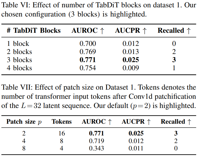
18.1 Transformer depth
| Blocks | AUROC | AUCPR | Recalled |
|---|---|---|---|
| 1 | 0.700 | 0.012 | 0 |
| 2 | 0.769 | 0.013 | 2 |
| 3 | 0.771 | 0.025 | 3 |
| 4 | 0.754 | 0.009 | 1 |
한 block은 capacity가 부족하고, 네 block은 작은 Dataset 1 training set에 overfit한 것으로 해석된다. 세 block이 최적이다.
하지만 depth를 Dataset 1의 anomaly metric으로 선택했다면 test anomaly label을 architecture selection에 사용했을 가능성이 있다. 별도의 validation anomaly가 없으므로 hyperparameter selection protocol을 명확히 할 필요가 있다.
18.2 Patch size
| Patch size | Transformer tokens | AUROC | AUCPR | Recalled |
|---|---|---|---|---|
| 2 | 16 | 0.771 | 0.025 | 3 |
| 4 | 8 | 0.719 | 0.012 | 2 |
| 8 | 4 | 0.343 | 0.011 | 0 |
Token 수가 16→8→4로 줄수록 성능이 크게 떨어진다. 저자들은 finer latent structure가 anomaly detection에 필요하다고 해석한다.
그러나 token이 원 test-program block과 직접 대응하지 않으므로, 이 결과는 “세밀한 test program localization”보다 더 긴 learned latent sequence가 Transformer capacity에 유리했다는 뜻으로 보는 편이 안전하다.
19. Root-cause Localization: 검증된 결과인가, 제안된 확장인가?
논문은 reverse diffusion reconstruction으로 원 feature별 residual을 계산하는 방식을 제안한다.
- Latent 에서 reverse process를 수행해 생성
- Decoder 로 원 feature space 복원
- Feature residual 계산
- 같은 test program 가 생성한 feature residual을 평균
이 결과를 test-flow heatmap으로 보여주면 leakage, timing, voltage 관련 어떤 program이 이상인지 engineer가 확인할 수 있다는 아이디어다.
중요한 평가
이 localization은 main anomaly detection experiment와 달리 다음이 보고되지 않았다.
- Feature-level ground truth와 localization accuracy
- 실제 anomaly example의 residual heatmap
- Process engineer의 root-cause validation
- Reverse step 수와 latency
- Stable feature ranking 여부
따라서 “interpretable failure localization을 제공했다”기보다 localization 가능한 scoring route를 수식으로 제안했다고 표현하는 것이 정확하다.
또한 dense autoencoder가 모든 input feature를 섞기 때문에 latent token residual 자체는 원 measurement와 직접 대응하지 않는다. 원 feature 해석에는 반드시 decoder와 feature grouping 단계가 필요하다.
Part V. 연구 기여와 비판적 분석
20. Step 03 - Challenge: 아이디어 구현에서 마주친 난관
20.1 수천 차원을 작은 latent로 줄이면서 anomaly evidence를 보존해야 한다
Compression이 너무 강하면 희소한 defect signal도 사라질 수 있다. 반대로 latent가 크면 diffusion과 Transformer 비용이 증가한다. 저자들은 128차원을 선택했지만 bottleneck size sensitivity는 제공하지 않는다.
20.2 Tabular feature에 token order를 만들어야 한다
Image와 달리 IC measurement에는 명백한 spatial adjacency가 없다. 저자들은 latent dimension을 1D sequence로 reshape하지만 semantic order의 근거가 약하다.
20.3 Wafer spatial variation과 defect를 분리해야 한다
Position effect를 제거하기만 하면 실제 location-dependent defect까지 약화될 수 있고, 무시하면 정상 edge die가 outlier가 된다. Within-wafer z-score와 die PE의 조합이 이 균형을 담당한다.
20.4 Diffusion score를 production speed에 맞춰야 한다
Full reverse sampling은 너무 비싸다. 저자들은 10개 mid-range timestep의 noise-prediction loss로 대체했지만, timestep 수와 speed-accuracy trade-off는 아직 검증되지 않았다.
20.5 극소수 anomaly로 model을 평가해야 한다
Dataset 1은 7개 anomaly뿐이다. 한 device의 ranking 변화가 recall과 AUCPR을 크게 바꾼다. Fixed seed 하나로는 uncertainty를 충분히 설명하기 어렵다.
21. Step 04 - Contribution: 해당 연구의 가치
Contribution 1. Raw IC parametric test를 위한 diffusion framework
저자 주장 기준으로, binary wafer map이나 equipment time series가 아니라 continuous-valued IC electrical test table에 diffusion model을 적용한 최초의 unsupervised framework를 제시했다.
Contribution 2. Latent diffusion으로 high dimension 문제를 완화
1,158~3,034개 feature를 128차원으로 줄인 뒤 diffusion해 raw-space TabDDPM보다 안정적인 성능을 보였다. Autoencoder 제거 시 Dataset 1 recall이 3에서 0으로 감소했다.
Contribution 3. Wafer position을 anomaly model에 명시적으로 조건화
Feature token PE와 die-coordinate PE를 분리해 test representation과 wafer geometry를 동시에 반영했다. Die PE 제거 시 AUROC가 0.234 감소해 spatial context의 중요성을 정량화했다.
Contribution 4. 생성 없이 diffusion loss만 사용하는 빠른 scoring
10개 timestep에서 noise prediction을 평가해 1,000-step reverse chain을 피했다. Diffusion model을 generator가 아니라 anomaly compatibility estimator로 사용한 실용적인 설계다.
Contribution 5. Yield-constrained metric을 도입
AUROC·AUCPR뿐 아니라 95% normal pass rate에서 실제 defect 몇 개를 회수하는지 보고했다. Model ranking을 제조 economics와 연결하려는 의미 있는 시도다.
Contribution 6. 폭넓은 baseline과 component ablation
Classical, deep, diffusion model을 폭넓게 비교하고 autoencoder, die PE, Transformer, depth, patch size의 효과를 분리했다.
22. Step 05 - Pros & Cons
| 구분 | 평가 |
|---|---|
| Pros - 실제 산업 문제 | Functional test를 통과한 latent defect라는 중요한 automotive IC 문제를 다룬다. |
| Pros - 실제 희소성 | 0.1~0.2% 수준 test prevalence에서 모델을 비교한다. |
| Pros - latent diffusion | Raw 3,000차원을 직접 확산하지 않아 계산과 conditioning을 개선한다. |
| Pros - spatial context | Die coordinate를 model에 넣어 정상 wafer variation을 처리한다. |
| Pros - 빠른 score | Reverse generation 없이 10회 noise prediction만 사용한다. |
| Pros - 생산 metric | Recalled@95% Yield로 false-positive/yield trade-off를 명시한다. |
| Pros - ablation | 주요 component와 depth·patch size를 정량 비교한다. |
| Cons - split leakage 위험 | 같은 lot·wafer의 die가 random train/test에 함께 들어갈 수 있다. |
| Cons - clean-train 가정 | Health label로 anomaly를 training에서 완전히 제외한다. |
| Cons - token semantics | Dense MLP latent를 reshape해 test-flow order가 명시적으로 보존되지 않는다. |
| Cons - Dataset 2 AUCPR | DiT1D가 최고가 아니며 절대 AUCPR도 0.0023으로 낮다. |
| Cons - anomaly 수 불일치 | Dataset 2의 41 anomalies와 본문의 7 anomalies가 충돌한다. |
| Cons - 95% yield | Normal 5% overkill은 실제 양산에 지나치게 클 수 있다. |
| Cons - localization 미검증 | Root-cause residual은 수식으로 제안했지만 정량·정성 결과가 없다. |
| Cons - 효율성 미측정 | A100에서 latency, throughput, memory, energy를 보고하지 않는다. |
| Cons - statistical uncertainty | Seed 42 한 번이며 confidence interval과 score variance가 없다. |
23. Step 06 - Takeaway: 내 연구에 적용해볼만한 포인트
23.1 Reconstruction error 대신 noise-prediction error를 anomaly signal로 사용할 수 있다
Diffusion model은 전체 sample을 복원하지 않아도 된다. 여러 noise level에서 normality를 얼마나 잘 설명하는지를 score로 사용할 수 있다.
Time-series window
    ↓ encoder
Latent patch tokens
    ↓ forward noise at selected t
Noise predictor
    ↓
Multi-timestep prediction error
    ↓
Normality discrepancy와 gated fusion
Reconstruction error가 local point deviation을 잡는다면 diffusion score는 latent distribution 적합도를 볼 수 있다. 두 signal의 상관관계와 보완성을 ablation해야 한다.
23.2 Context를 anomaly로 오인하지 않도록 별도 embedding으로 조건화한다
이 논문의 die PE는 “정상 context variation을 model이 설명하게 만든다”는 좋은 설계 원리다.
시계열에서는 다음 context가 대응된다.
- tool 또는 chamber ID
- recipe
- operating mode
- maintenance state
- batch/lot
- seasonal·shift context
Context를 raw sensor와 단순 concatenate하기보다 gated embedding으로 조건화하고, w/o context, shuffled context, wrong context ablation을 수행하면 의미 대응의 중요성을 검증할 수 있다.
23.3 Tokenization은 reshape가 아니라 semantic group을 보존해야 한다
이 논문의 가장 아쉬운 점은 learned latent dimension을 그대로 reshape한다는 것이다.
- sensor-group token
- temporal patch token
- process-phase token
- test-program token
- variable-cluster token
Token 위치와 실제 domain unit이 대응하면 attention과 residual localization을 해석하기 쉬워진다.
23.4 Extreme imbalance에서는 AUROC보다 AUPR와 operating point를 우선한다
Dataset 2에서 AUROC는 DiT1D가 최고지만 AUCPR은 다른 method가 더 높다.
- AUPR/V-PR
- Range-F1/Affiliation-F1
- Recall at fixed false-positive rate
- False alarms/hour
- Yield 또는 review budget에서의 recall
23.5 Fixed threshold가 아니라 risk budget으로 평가한다
반도체에서는 “score > 0.5”보다 다음 질문이 더 실용적이다.
하루 100개만 추가 검사할 수 있다면 실제 defect를 몇 개 회수하는가?
이를 일반화하면 다음 metric을 사용할 수 있다.
- Recall@Top-K
- Precision@inspection budget
- Recall@99.9% yield
- Cost-weighted utility
- Expected field-failure reduction
23.6 Interpretation은 원 feature까지 역매핑되어야 한다
Latent token heatmap만으로는 process engineer가 조치하기 어렵다. Feature·sensor·test program으로 돌아가는 decoder 또는 attribution map이 필요하다. 그리고 explanation quality도 ground truth root cause나 expert agreement로 평가해야 한다.
23.7 Multi-seed와 bootstrap이 특히 중요하다
Anomaly가 7개라면 한 sample의 ranking이 recall을 14.3%p 바꾼다. 최소한 다음을 권장한다.
- 여러 train seed의 mean±std
- Test anomaly bootstrap confidence interval
- Noise draw 반복에 따른 score variance
- Top-ranked device의 rank stability
- Die PE effect의 lot/wafer별 일관성
24. Step 07 - Limitation: 후속 연구의 기회
24.1 Lot·wafer·time 단위 external split
Random die split 대신 다음 평가가 필요하다.
- Train wafer와 test wafer 완전 분리
- Train lot와 test lot 완전 분리
- 이전 release로 train, 다음 release로 test
- 시간 순서 기반 prospective validation
이렇게 해야 die PE가 wafer pattern을 memorize한 것이 아니라 새로운 wafer의 spatial variation을 generalize했는지 알 수 있다.
Within-wafer z-score도 각 split 안에서 독립적으로 계산하고, prospective setting에서는 현재까지 관측된 die 또는 과거 정상 wafer의 statistic만 사용해야 한다. 전체 wafer의 train·test die를 함께 사용한 normalization과 비교해 leakage 영향을 분리할 필요가 있다.
24.2 Contaminated normal training
실제 deployment에서는 latent defect가 training data에 섞여 있을 수 있다. Contamination 0.01%, 0.1%, 0.5%, 1%에서 성능을 비교하고 robust loss, trimming, iterative cleaning을 적용해야 한다.
24.3 더 높은 yield operating point
95%뿐 아니라 99%, 99.9%, 99.99% yield에서 recall을 보고해야 한다. Product cost와 field-return cost를 기반으로 expected economic utility를 계산하면 산업 기여가 더 명확해진다.
24.4 Semantic tokenization
Test program별 contiguous feature block을 직접 token으로 만들고 program ID embedding을 추가할 수 있다.
Program 1 measurements → token 1
Program 2 measurements → token 2
...
Program P measurements → token P
이렇게 하면 attention과 reconstruction residual이 test flow 의미와 직접 대응한다.
24.5 Timestep와 inference budget ablation
다음을 비교해야 한다.
- Single timestep vs. 3/5/10/20 timesteps
- Low/mid/high noise range
- Deterministic fixed noise vs. multiple random draws
- Score accuracy vs. latency Pareto curve
24.6 Localization validation
실제 defect에 대해 다음을 평가해야 한다.
- Top-k feature hit rate
- Test-program-level recall
- Engineer-rated explanation usefulness
- Known failure mechanism과 residual profile의 일치도
- Root-cause diagnosis time 감소
24.7 Baseline tuning과 simple model 비교
Published default만 쓴 baseline보다 동일 validation budget으로 tuning해야 공정하다. 또한 4M-parameter DiT가 필요한지 확인하기 위해 다음이 필요하다.
- Latent PCA + Mahalanobis distance
- Autoencoder latent KNN/LOF
- Masked autoencoder
- Latent MLP denoiser
- Small Transformer without diffusion
- Energy-based model
24.8 실제 deployment benchmark
A100이 아니라 production server 또는 edge system에서 다음을 측정해야 한다.
- die당 latency
- wafer당 screening time
- throughput
- peak memory
- 10-pass scoring cost
- power와 energy/die
- decoder localization을 포함한 expert-analysis latency
24.9 Dataset 2 label accounting 수정
41 anomaly와 7 confirmed anomaly의 관계, train/test 분포, Recalled metric의 denominator를 명확히 공개해야 한다. 이 정보가 없으면 7이라는 결과를 recall 17.1%로 볼지 100%로 볼지 결정할 수 없다.
Part VI. 연구 Insight와 최종 정리
25. 논문을 읽고 얻은 Insight
Insight 1. Diffusion은 생성보다 density compatibility test로 더 실용적일 수 있다
Industrial anomaly detection에서는 예쁜 sample을 생성할 필요가 없다. Normal distribution에서 noise를 얼마나 잘 예측하는지만으로 빠른 score를 만들 수 있다.
Insight 2. Context embedding이 anomaly detector의 핵심일 수 있다
Die PE 제거 시 AUROC가 0.234 감소했다. Model backbone만큼 “무엇을 정상 variation으로 설명할 것인가”가 중요하다.
Insight 3. High-dimensional anomaly detection에서는 압축 방식이 backbone보다 중요할 수 있다
Autoencoder 제거 시 recall이 3에서 0으로 떨어졌다. Raw-space diffusion보다 representation conditioning이 우선이다.
Insight 4. Token이 있다고 모두 semantic token은 아니다
Dense latent reshape는 Transformer input sequence를 만들지만, token과 실제 test program의 대응을 보장하지 않는다. Interpretability claim에는 explicit alignment가 필요하다.
Insight 5. Relative SOTA와 production usefulness는 다르다
Dataset 1 AUCPR은 random보다 11배 높지만 절대값은 0.025다. 95% yield에서 3개 defect를 찾는 대신 약 156개 normal die를 추가 선별한다. 좋은 연구 결과지만 곧바로 production-ready라는 뜻은 아니다.
Insight 6. Metric마다 서로 다른 model이 이길 수 있다
Dataset 2에서는 DiT1D가 AUROC와 fixed-yield recall에서 이기지만 DTE-IG가 AUCPR에서 이긴다. Model 선택은 실제 operating constraint로 결정해야 한다.
Insight 7. Interpretability는 가능성보다 검증이 중요하다
Feature residual 수식이 있다고 root-cause analysis가 완성되는 것은 아니다. 실제 engineer가 원인을 더 빨리 찾았는지까지 평가해야 한다.
26. 7-Step 최종 정리
| Step | 항목 | 이 논문에 대한 답 |
|---|---|---|
| 01 | Problem | Latent defect는 극도로 희소하고 IC test는 수천 차원이며, wafer spatial variation과 defect를 구분하면서 normal overkill도 최소화해야 한다. |
| 02 | Idea | IC measurement를 128차원 latent token으로 압축하고 die 위치를 조건으로 넣은 DiT1D의 multi-timestep noise-prediction error를 anomaly score로 사용한다. |
| 03 | Challenge | 고차원 압축, tabular tokenization, wafer context modelling, diffusion inference 비용, 7개 수준의 anomaly 평가가 어렵다. |
| 04 | Contribution | Raw IC parametric test용 latent diffusion framework, two-level PE, 10-pass scoring, yield-constrained 평가를 제안하고 Dataset 1에서 AUROC 0.771·AUCPR 0.025·3개 anomaly 회수를 달성했다. |
| 05 | Pros & Cons | 실제 산업 희소성과 spatial context를 잘 반영하지만 random die split, clean-train 가정, 약한 token semantics, Dataset 2 수치 불일치, 미검증 localization이 약점이다. |
| 06 | Takeaway | Normal context를 별도 embedding으로 조건화하고, semantic token을 유지하며, AUPR와 fixed-risk operating point 및 multi-seed uncertainty를 우선 평가해야 한다. |
| 07 | Limitation | Lot/wafer external validation, contamination robustness, 99.9% yield 평가, timestep-efficiency ablation, root-cause localization 검증, 실제 deployment가 후속 연구 기회다. |
27. Conclusion
Diffuse to Detect는 functional test를 통과한 latent defect를 찾기 위해 diffusion model을 IC parametric test에 맞게 재설계한 연구다. 수천 차원의 raw measurement를 128차원 latent로 줄이고, 이를 1D token sequence로 reshape한 뒤 feature-position PE와 wafer die-coordinate PE를 더한다. 정상 die만으로 학습된 3-block Diffusion Transformer는 여러 중간 timestep에서 주입된 Gaussian noise를 예측하며, prediction MSE의 평균이 anomaly score가 된다.
Dataset 1에서는 AUROC 0.771, AUCPR 0.0250, Recalled@95% Yield 3으로 모든 비교 metric에서 가장 좋은 결과를 보였다. 특히 AUCPR은 random level의 약 11배, second-best의 약 4배다. Dataset 2에서는 AUROC 0.639와 Recalled 7로 가장 좋았지만 AUCPR 0.0023은 DTE-IG 0.0055보다 낮았다. 따라서 두 dataset 모두에서 모든 metric을 지배한 것은 아니다.
Ablation은 세 설계의 필요성을 보여준다. Autoencoder를 제거하면 recall이 0이 되고, die PE를 제거하면 AUROC가 0.234 감소하며, Transformer를 MLP denoiser로 바꾸면 recall이 3에서 1로 줄어든다. 이는 high-dimensional compression, spatial conditioning, inter-token modeling이 모두 기여했음을 시사한다.
다만 논문의 “structured semantic token”과 “interpretable localization” 주장은 아직 신중하게 읽어야 한다. Dense MLP encoder가 원 feature를 전역적으로 섞은 뒤 latent dimension을 reshape하므로 token이 test program order와 직접 대응하지 않는다. Feature-level root-cause residual은 수식으로 제안됐지만 실제 defect heatmap이나 engineer validation은 없다.
또한 random die split은 같은 wafer·lot 정보가 train과 test에 함께 들어갈 가능성이 있고, training anomaly를 label로 완전히 제거한 clean setting만 평가한다. Dataset 2의 41 anomaly와 본문의 7 anomaly 불일치, 단일 seed, 95% yield라는 큰 overkill budget, A100에서 실제 throughput 미보고도 production-ready claim을 제한한다.
그럼에도 이 논문이 주는 방향은 분명하다.
극희소 산업 anomaly를 찾기 위해서는 더 큰 generative model보다, 정상 variation의 context를 정확히 조건화하고 고차원 신호를 안정적인 latent space로 바꾸며 실제 screening budget에서 ranking을 평가하는 설계가 중요하다.
향후 semantic test-program token, lot·wafer external split, contaminated training, 99.9% 이상의 yield constraint, 실제 root-cause validation까지 연결한다면 Diffuse to Detect는 automotive semiconductor quality control에 훨씬 가까운 framework가 될 수 있다.