머신러닝 알고리즘
머신러닝의 알고리즘 종류는 크게 3가지로 나눌 수 있다.
- 지도학습 (Supervised Learning)
- 비지도학습 (Unsupervised Learning)
- 강화학습 (Reinforcement Learning)
지도학습의 대표 알고리즘
- 분류(Classification) : 예측해야할 데이터가 범주형(categorical) 변수일때 분류 라고 함
- 회귀(Regression) : 예측해야할 데이터가 연속적인 값 일때 회귀 라고 함
- 예측(Forecasting) : 과거 및 현재 데이터를 기반으로 미래를 예측하는 과정 예를 들어 올해와 전년도 매출을 기반으로 내년도 매출을 추산하는 것.
비지도학습의 대표 알고리즘
- 클러스터링 : 특정 기준에 따라 유사한 데이터끼리 그룹화함
- 차원축소 : 고려해야할 변수를 줄이는 작업, 변수와 대상간 진정한 관계를 도출하기 용이
참고링크- 최적의 ‘머신러닝 알고리즘’을 고르기 위한 치트키
강화학습
강화학습은 앞에서 언급한 지도학습, 비지도학습과는 다른 종류의 알고리즘이다. 학습하는 시스템을 에이전트라고 하고, 환경을 관찰해서 에이전트가 스스로 행동하게 한다. 모델은 그 결과로 특정 보상을 받아 이 보상을 최대화하도록 학습한다.
- 에이전트(Agent) : 학습 주체 (혹은 actor, controller)
- 환경(Environment) : 에이전트에게 주어진 환경, 상황, 조건
- 행동(Action) : 환경으로부터 주어진 정보를 바탕으로 에이전트가 판단한 행동
- 보상(Reward) : 행동에 대한 보상을 머신러닝 엔지니어가 설계
대표 알고리즘
- Monte Carlo methods
- Q-Learning
- Policy Gradient methods
사이킷런을 이용한 머신러닝 구현
Scikit-Learn은 sciPy와 Toolkit을 합쳐서 만들어졌다. 알고리즘은 파이썬 클래스로 구현되어 있고, 데이터셋은 NumPy의 ndarray, Pandas의 DataFrame, SciPy의 Sparse Matrix를 이용해 나타낼 수 있다. 그리고 훈련과 예측 등 머신러닝 모델을 다룰 때는 CoreAPI라고 불리는 fit(), transfomer(), predict()과 같은 함수들을 이용한다.
주로 사용하는 API
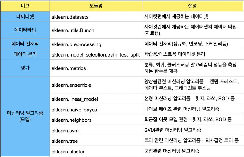
데이터 표현법
사이킷런에서는 데이터 표현 방식을 보통 2가지로 나타냅니다. 바로 특성 행렬(Feature Matrix) 과 타겟 벡터(Target Vector) 이다.
[출처: https://jakevdp.github.io/PythonDataScienceHandbook/06.00-figure-code.html#Features-and-Labels-Grid]
특성 행렬(Feature Matrix)
- 입력 데이터를 의미
- 특성(feature) : 데이터에서 수치 값, 이산 값, 불리언 값으로 표현되는 개별 관측치를 의미한다. 특성 행렬에서는 열에 해당하는 값이다.
- 표본(sample) : 각 입력 데이터, 특성 행렬에서는 행에 해당하는 값이다.
n_samples: 행의 개수(표본의 개수)n_features: 열의 개수(특성의 개수)X: 통상 특성 행렬은 변수명 X로 표기
[n_samples, n_features]은 [행, 열] 형태의 2차원 배열 구조를 사용하며 이는 NumPy의 ndarray, Pandas의 DataFrame, SciPy의 Sparse Matrix를 사용하여 나타낼 수 있다.
타겟 벡터 (Target Vector)
- 입력 데이터의 라벨(정답)을 의미
- 목표(Target) : 라벨, 타겟값, 목표값이라고도 부르며 특성 행렬(Feature Matrix)로부터 예측하고자 하는 것을 말한다.
n_samples: 벡터의 길이(라벨의 개수)- 타겟 벡터에서
n_features는 없다. y: 통상 타겟 벡터는 변수명 y로 표기- 타겟 벡터는 보통 1차원 벡터로 나타내며, 이는 NumPy의 ndarray, Pandas의 Series를 사용하여 나타낼 수 있다.
- 단, 타겟 벡터는 경우에 따라 1차원으로 나타내지 않을 수도 있다.
❗️특성 행렬 X의 n_samples와 타겟 벡터 y의 n_samples는 동일해야 한다.
회귀모델
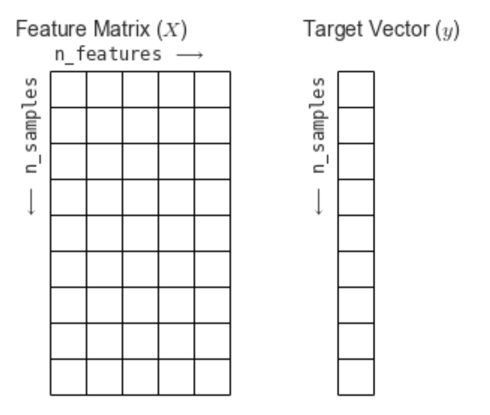
회귀 모델을 이용해 데이터를 예측하는 모델을 만들어 보자.
import numpy as np
import matplotlib.pyplot as plt
r = np.random.RandomState(10)
x = 10 * r.rand(100)
y = 2 * x - 3 * r.rand(100)
plt.scatter(x,y)
/-----------------------------/
# 출력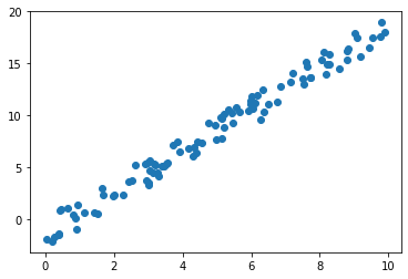
입력 데이터 x와 정답 데이터 y의 모양을 확인해 보자.
print(x.shape)
print(y.shape)
/------------/
# 출력
(100,)
(100,)
1차원 벡터 데이터를 가지고 선형 회귀 모델을 돌려보자.
from sklearn.linear_model import LinearRegression
model = LinearRegression()
model.fit(x, y)
/-----------------------------------------------/
# 출력
ValueError: Expected 2D array, got 1D array instead:x데이터가 행렬이 아니라서 에러가 발생한다. numpy의 ndarray타입이니 reshape()를 사용하면 된다.
X = x.reshape(100,1)
model.fit(X,y)
/------------------/
# 출력
LinearRegression()
학습한 모델을 가지고 예측해보자.
x_new = np.linspace(-1, 11, 100)
X_new = x_new.reshape(100,1)
y_new = model.predict(X_new)
y_new
/------------------------------/
# 출력
array([-3.5035171 , -3.25845808, -3.01339905, -2.76834003, -2.52328101,
       -2.27822198, -2.03316296, -1.78810393, -1.54304491, -1.29798588,
       -1.05292686, -0.80786783, -0.56280881, -0.31774978, -0.07269076,
        0.17236826,  0.41742729,  0.66248631,  0.90754534,  1.15260436,
        1.39766339,  1.64272241,  1.88778144,  2.13284046,  2.37789949,
        2.62295851,  2.86801754,  3.11307656,  3.35813558,  3.60319461,
        3.84825363,  4.09331266,  4.33837168,  4.58343071,  4.82848973,
        5.07354876,  5.31860778,  5.56366681,  5.80872583,  6.05378485,
        6.29884388,  6.5439029 ,  6.78896193,  7.03402095,  7.27907998,
        7.524139  ,  7.76919803,  8.01425705,  8.25931608,  8.5043751 ,
        8.74943413,  8.99449315,  9.23955217,  9.4846112 ,  9.72967022,
        9.97472925, 10.21978827, 10.4648473 , 10.70990632, 10.95496535,
       11.20002437, 11.4450834 , 11.69014242, 11.93520144, 12.18026047,
       12.42531949, 12.67037852, 12.91543754, 13.16049657, 13.40555559,
       13.65061462, 13.89567364, 14.14073267, 14.38579169, 14.63085072,
       14.87590974, 15.12096876, 15.36602779, 15.61108681, 15.85614584,
       16.10120486, 16.34626389, 16.59132291, 16.83638194, 17.08144096,
       17.32649999, 17.57155901, 17.81661803, 18.06167706, 18.30673608,
       18.55179511, 18.79685413, 19.04191316, 19.28697218, 19.53203121,
       19.77709023, 20.02214926, 20.26720828, 20.51226731, 20.75732633])
Tip!
reshape()함수에서 나머지 숫자를 -1로 넣으면 자동으로 남은 숫자를 계산해 준다.X_ = x_new.reshape(-1,1) X_.shape /----------------------/ # 출력 (100, 1)
회귀 모델의 경우 RMSE(Root Mean Square Error) 를 사용해 성능을 평가한다.
from sklearn.metrics import mean_squared_error

error = error = np.sqrt(mean_squared_error(y,y_new))

print(error)
/--------------------------------------------------/
# 출력
9.299028215052264
직관적으로 확인하기 위해 그래프로 그려보자.
plt.scatter(x, y, label='input data')
plt.plot(X_new, y_new, color='red', label='regression line')
/----------------------------------------------------------/
# 출력
데이터셋 모듈
공식 문서
사이킷런은 데이터셋을 모듈로 제공하고 있다.
from sklearn.datasets import load_wine
data = load_wine()
type(data)
/------------------------------------/
# 출력
sklearn.utils.BunchBunch는 파이썬의 딕셔너리와 유사한 형태의 데이터 타입이다.
data.keys()
/---------/
# 출력
dict_keys(['data', 'target', 'frame', 'target_names', 'DESCR', 'feature_names'])
각 항목별로 의미하는 것이 무엇인지 알아보자.
1) data
키값 data는 특성 행렬이다.
data.data
/-------/
# 출력
array([[1.423e+01, 1.710e+00, 2.430e+00, ..., 1.040e+00, 3.920e+00,
        1.065e+03],
       [1.320e+01, 1.780e+00, 2.140e+00, ..., 1.050e+00, 3.400e+00,
        1.050e+03],
       [1.316e+01, 2.360e+00, 2.670e+00, ..., 1.030e+00, 3.170e+00,
        1.185e+03],
       ...,
       [1.327e+01, 4.280e+00, 2.260e+00, ..., 5.900e-01, 1.560e+00,
        8.350e+02],
       [1.317e+01, 2.590e+00, 2.370e+00, ..., 6.000e-01, 1.620e+00,
        8.400e+02],
       [1.413e+01, 4.100e+00, 2.740e+00, ..., 6.100e-01, 1.600e+00,
        5.600e+02]])
특성 행렬은 2차원이며 행에는 데이터의 개수(n_samples)가 열에는 특성의 개수(n_features)가 들어있다.
data.data.shape
/-------------/
# 출력
(178, 13)
특성이 13개, 데이터가 178개인 특성 행렬이 나온다.
2) target
print(data.target)
data.target.shape
/----------------/
[0 0 0 0 0 0 0 0 0 0 0 0 0 0 0 0 0 0 0 0 0 0 0 0 0 0 0 0 0 0 0 0 0 0 0 0 0
 0 0 0 0 0 0 0 0 0 0 0 0 0 0 0 0 0 0 0 0 0 0 1 1 1 1 1 1 1 1 1 1 1 1 1 1 1
 1 1 1 1 1 1 1 1 1 1 1 1 1 1 1 1 1 1 1 1 1 1 1 1 1 1 1 1 1 1 1 1 1 1 1 1 1
 1 1 1 1 1 1 1 1 1 1 1 1 1 1 1 1 1 1 1 2 2 2 2 2 2 2 2 2 2 2 2 2 2 2 2 2 2
 2 2 2 2 2 2 2 2 2 2 2 2 2 2 2 2 2 2 2 2 2 2 2 2 2 2 2 2 2 2]

(178,)
3) feature_names
data.feature_names
/----------------/
# 출력
['alcohol',
 'malic_acid',
 'ash',
 'alcalinity_of_ash',
 'magnesium',
 'total_phenols',
 'flavanoids',
 'nonflavanoid_phenols',
 'proanthocyanins',
 'color_intensity',
 'hue',
 'od280/od315_of_diluted_wines',
 'proline']
4) target_names
target_names는 분류하고자 하는 대상이다.
data.target_names
/---------------/
# 출력
array(['class_0', 'class_1', 'class_2'], dtype='<U7')
데이터를 각각 class_0과 class_1, class_2로 분류한다는 뜻이다.
5) DESCR
DESCR은 describe의 약자로 데이터에 대한 설명이다.
print(data.DESCR)
/---------------/
# 출력
.. _wine_dataset:

Wine recognition dataset
------------------------

**Data Set Characteristics:**

    :Number of Instances: 178 (50 in each of three classes)
    :Number of Attributes: 13 numeric, predictive attributes and the class
    :Attribute Information:
 		- Alcohol
 		- Malic acid
 		- Ash
		- Alcalinity of ash
 		- Magnesium
		- Total phenols
 		- Flavanoids
 		- Nonflavanoid phenols
 		- Proanthocyanins
		- Color intensity
 		- Hue
 		- OD280/OD315 of diluted wines
 		- Proline

    - class:
            - class_0
            - class_1
            - class_2

    :Summary Statistics:

    ============================= ==== ===== ======= =====
                                   Min   Max   Mean     SD
    ============================= ==== ===== ======= =====
    Alcohol:                      11.0  14.8    13.0   0.8
    Malic Acid:                   0.74  5.80    2.34  1.12
    Ash:                          1.36  3.23    2.36  0.27
    Alcalinity of Ash:            10.6  30.0    19.5   3.3
    Magnesium:                    70.0 162.0    99.7  14.3
    Total Phenols:                0.98  3.88    2.29  0.63
    Flavanoids:                   0.34  5.08    2.03  1.00
    Nonflavanoid Phenols:         0.13  0.66    0.36  0.12
    Proanthocyanins:              0.41  3.58    1.59  0.57
    Colour Intensity:              1.3  13.0     5.1   2.3
    Hue:                          0.48  1.71    0.96  0.23
    OD280/OD315 of diluted wines: 1.27  4.00    2.61  0.71
    Proline:                       278  1680     746   315
    ============================= ==== ===== ======= =====

    :Missing Attribute Values: None
    :Class Distribution: class_0 (59), class_1 (71), class_2 (48)
    :Creator: R.A. Fisher
    :Donor: Michael Marshall (MARSHALL%PLU@io.arc.nasa.gov)
    :Date: July, 1988

This is a copy of UCI ML Wine recognition datasets.
https://archive.ics.uci.edu/ml/machine-learning-databases/wine/wine.data

The data is the results of a chemical analysis of wines grown in the same
region in Italy by three different cultivators. There are thirteen different
measurements taken for different constituents found in the three types of
wine.

Original Owners:

Forina, M. et al, PARVUS -
An Extendible Package for Data Exploration, Classification and Correlation.
Institute of Pharmaceutical and Food Analysis and Technologies,
Via Brigata Salerno, 16147 Genoa, Italy.

Citation:

Lichman, M. (2013). UCI Machine Learning Repository
[https://archive.ics.uci.edu/ml]. Irvine, CA: University of California,
School of Information and Computer Science.

.. topic:: References

  (1) S. Aeberhard, D. Coomans and O. de Vel,
  Comparison of Classifiers in High Dimensional Settings,
  Tech. Rep. no. 92-02, (1992), Dept. of Computer Science and Dept. of
  Mathematics and Statistics, James Cook University of North Queensland.
  (Also submitted to Technometrics).

  The data was used with many others for comparing various
  classifiers. The classes are separable, though only RDA
  has achieved 100% correct classification.
  (RDA : 100%, QDA 99.4%, LDA 98.9%, 1NN 96.1% (z-transformed data))
  (All results using the leave-one-out technique)

  (2) S. Aeberhard, D. Coomans and O. de Vel,
  "THE CLASSIFICATION PERFORMANCE OF RDA"
  Tech. Rep. no. 92-01, (1992), Dept. of Computer Science and Dept. of
  Mathematics and Statistics, James Cook University of North Queensland.
  (Also submitted to Journal of Chemometrics).
분류 모델 만들기
특성 행렬을 Pandas의 DataFrame으로 나타낼 수 있다고 했다.
import pandas as pd

pd.DataFrame(data.data, columns=data.feature_names).head()
/--------------------------------------------------------/
# 출력
	alcohol	malic_acid	ash	alcalinity_of_ash	magnesium	total_phenols	flavanoids	nonflavanoid_phenols	proanthocyanins	color_intensity	hue	od280/od315_of_diluted_wines	proline
0	14.23	1.71		2.43	15.6			127.0		2.80		3.06		0.28			2.29		5.64		1.04	3.92				1065.0
1	13.20	1.78		2.14	11.2			100.0		2.65		2.76		0.26			1.28		4.38		1.05	3.40				1050.0
2	13.16	2.36		2.67	18.6			101.0		2.80		3.24		0.30			2.81		5.68		1.03	3.17				1185.0
3	14.37	1.95		2.50	16.8			113.0		3.85		3.49		0.24			2.18		7.80		0.86	3.45				1480.0
4	13.24	2.59		2.87	21.0			118.0		2.80		2.69		0.39			1.82		4.32		1.04	2.93				735.0
모델 생성
분류 문제이므로 RandomForestClassifier을 이용해보자.
X = data.data
y = data.target
from sklearn.ensemble import RandomForestClassifier
model = RandomForestClassifier()
model.fit(X, y)
/--------------------------------------------------/
# 출력
RandomForestClassifier()
예측 후 성능평가를 해보자.
from sklearn.metrics import accuracy_score
from sklearn.metrics import classification_report

y_pred = model.predict(X)

# 타겟 벡터 즉 라벨인 변수명 y와 예측값 y_pred을 각각 인자로 넣는다.
print(classification_report(y, y_pred))
# 정확도를 출력.
print("accuracy = ", accuracy_score(y, y_pred))
/----------------------------------------------------------/
# 출력
              precision    recall  f1-score   support

           0       1.00      1.00      1.00        59
           1       1.00      1.00      1.00        71
           2       1.00      1.00      1.00        48

    accuracy                           1.00       178
   macro avg       1.00      1.00      1.00       178
weighted avg       1.00      1.00      1.00       178

accuracy =  1.0
정확도가 100%가 나온것을 확인할 수 있다. 이렇게 나오는 이유가 뭘까? 이후에 나오는 내용에서 다룰 예정이다.
Estimator
데이터셋을 기반으로 머신러닝 모델의 파라미터를 추정하는 객체를 Estimator라고 한다. 사이킷런의 모든 머신러닝 모델은 Estimator라는 파이썬 클래스로 구현되어 있다. 추정을 하는 과정 즉, 훈련은 Estimator의 fit()메서드를 통해 이루어지고, 예측은 predict()메서드를 통해 이루어진다.
와인 분류 문제를 그림으로 표현하면 아래와 같다.
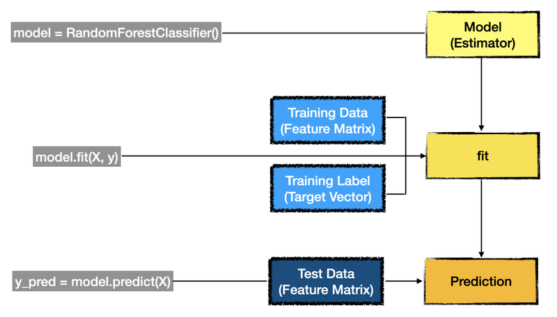
훈련 데이터와 테스트 데이터 분리하기
우리는 와인 분류 문제에서 정확도가 100%가 나온 것을 알고 있다. 위의 그림을 보면 fit()과 prediction()메서드에 인자로 각기 다른 데이터가 들어가야 하는 것을 확인할 수 있다.
위에서 진행한 모델 훈련에는 사용되는 데이터(특성 행렬)와 예측에 사용되는 데이터(특성 행렬)에 같은 값을 넣었다. 즉, 동일한 데이터로 훈련과 예측을 하니 정확도가 100% 로 나왔다.
위의 Estimator 이미지를 보면 훈련과 예측에 각기 다른 데이터를 사용해야한다. 그럼 이제 직접 분리해보자.
from sklearn.datasets import load_wine
data = load_wine()
print(data.data.shape)
print(data.target.shape)
/------------------------------------/
# 출력
(178, 13)
(178,)
보통 훈련 데이터와 테스트 데이터의 비율은 8:2로 설정한다. 전체 데이터의 개수는 178개다. 8 대 2로 특성 행렬과 타겟 벡터를 나누어 보도록 하자. 데이터의 개수이므로 정수만 가능하다. 178개의 80%면 142.4이지만 정수로 표현해 142개, 그리고 훈련 데이터는 나머지 36개로 나누어 보자.
슬라이싱을 이용해 나눠보자.
X_train = data.data[:142]
X_test = data.data[142:]
y_train = data.target[:142]
y_test = data.target[142:]
print(X_train.shape, X_test.shape)
print(y_train.shape, y_test.shape)
/--------------------------------/
# 출력
(142, 13) (36, 13)
(142,) (36,)
나눠진 데이터는 학습이 잘 될까?
from sklearn.ensemble import RandomForestClassifier
model = RandomForestClassifier()
model.fit(X_train, y_train)
/-------------------------------------------------/
# 출력
RandomForestClassifier()
from sklearn.metrics import accuracy_score
y_pred = model.predict(X_test)
print("정답률=", accuracy_score(y_test, y_pred))
/---------------------------------------------/
# 출력
정답률= 0.9722222222222222정상적으로 잘 학습되는 것을 확인할 수 있다.
하지만 슬라이싱으로 하는 것은 많이 귀찮을 수 있다.
이에 사이킷런에서 데이터 분리를 위한 API를 제공한다. model_selection의 train_test_split() 함수이다.
from sklearn.model_selection import train_test_split

result = train_test_split(X, y, test_size=0.2, random_state=42)
print(type(result))
print(len(result))
print(result[0].shape)
print(result[1].shape)
print(result[2].shape)
print(result[3].shape)
/-------------------------------------------------------------/
# 출력
<class 'list'>
4
(142, 13)
(36, 13)
(142,)
(36,)train_test_split()은 반환값으로 4개의 원소로 이루어진 list를 반환한다.
보통은 이 함수를 unpacking해서 사용한다.
X_train, X_test, y_train, y_test = train_test_split(X, y, test_size=0.2, random_state=42)