B-cos Networks: Alignment is All We Need for Interpretability
Author
Abstract
This paper proposed a weight-input alignment method that replaces the linear transform of the existing DNN architecture with the B-cos proposed in this paper to increase the interpretability. B-cos is designed to be easily integrated into common models such as VGG, ResNet, InceptionNet, and DenseNet. The code is available at github.com/moboehle/B-cos.
Introduction
B-cos transform can improve the interpretability of neural networks. By promoting weight-input alignment, we provide descriptions that highlight task-relevant patterns in the input data. In particular, the B-cos transform can provide a reliable summary of any sequence of B-cos through a single linear transformation. This shows that it can explain not only the output of the model, but also the neurons of any intermediate network layer. Also, this method can easily be integrated into various commonly used DNNs including InceptionNet [1], ResNet [2], VGG [3], and DenseNet [4] models, whilst maintaining similar performance.
B-cos neural networks
The B-cos transform
Typically, each neuron in a DNN calculates the dot product between weight w and input x. Here, ∠(x, w) returns the angle between the vectors x and w. In this work, the research seeks to improve the interpretability of DNNs by weight-input alignment during optimization.
Here, B is a hyperparameter, the hat-operator scales wb to unit norm, and sgn denotes the sign function. Here, the difference between Equation (1) is the blue part. This small section is important for three reasons.
First, they bound the output of B-cos neurons. As becomes clear from Equation (1), equality in Equation (4) is only achieved if x and w are collinear (aligned)
Second, by increasing B, we can limit the output of unordered weights. In addition, each B-cos unit can only generate an output close to the maximum (||X||) for a small range of angular deviations from x. Using these two properties together can significantly change the optimal value of the weight w. Figure 2, shows that increasing the value of B affects a simple linear classification problem. Especially if B has a large value, Equation (4) and (5) shift the optimality in the optimization problem. The optimal weights align with the red data clusters in Figure. 2, regardless of other classes. the B-cos transform enables similarity-based explanations, unlike conventional highly task-dependent linear classification. Finally, B-cos retains important properties of linear transformations.
Simple (convolutional) B-cos networks
This section describes how to construct a simple DNN based on the B-cos transform. And then, summarize the network output with a linear transform. Finally, show why this transform matches the discriminant input pattern in the classification task.
The B-cos transform is designed as a replacement for the linear transform. So, it can be used in exactly the same way.
lj is layer j with parameters wkj for neuron k in layer j, and θ the collection of all model parameters.
These models typically compute as in Equation 7. In addition, the nonlinear activation function φ sequentially models the nonlinear relationship of several layers as follows.
The only difference here is that the dot product is replaced by the B-cos transform. Expressing this as a matrix form,
All operations are element-wise, and c(aj, Wcj) calculates the cosine similarity. The hat operator scales Wcj rows to unit norm. When B>1, layer transform I * j is non-linear. As a result, the nonlinear activation function φ is not necessary for B-cos networks to model nonlinear relationships.
Computing explanations for B-cos networks
The Equation (9) B-cos layer effectively calculates the input-dependent linear transform.
Here, The dot scales the row of the right matrix by the scalar entry of the left vector. Therefore, the output of the B-cos network (Equation 8) is effectively calculated as:
It also can be reduce by single transform, the output f ∗ (x; θ) can be written as
Thus, W1→L(x) faithfully summarizes the network computation (Equation (8)) into a single linear transformation (Equation (13)). Rows in W1→L or contributions according to W1→L coming from individual input dimensions can directly visualize to explain activations (e.g. class logits) (Figure (1), (10)). The resulting spatial contribution map is used to quantitatively evaluate explanations. Specifically, the input contribution slj(x) to neuron j in layer l for input x is given by
[W1→l]j denotes the j row of matrix W1→l.
Optimising B-cos networks for classification
The output of each neuron and each layer are limited as in Equations (4),(9). In addition, the entire B-cos network can reach the upper boundary only when the units of each layer reach the upper limit. In particular, each unit can only reach the maximum value if their inputs are aligned. Therefore, if we optimize a B-cos network to maximize the output for a set of inputs, the model weights will be optimized by align the inputs.
This paper use BCE (Binary Cross Entropy) loss to optimize the classification.
Here, σ denotes the sigmoid function, b a bias, and θ the model parameters.
By increasing B, the output of badly ordered weights in each layer can be reduced. This is because the strength of the layer's output decreases, so the strength for badly aligned weights decreases, which in turn increases the alignment strength. (increase of B -> higher sort)MaxOut to increase modelling capacity
this research model every neuron in a B-cos network by 2 B-cos transforms of which the maximaly activated neurons is forwarded:
In order to forward a large signal, one MaxOut[5] unit still needs to have at least one weight vector that highly aligns with a given input. Also, the alignment pressure is thus maintained during optimisation. Networks with MaxOut operations were easier to optimize.
Advanced B-cos network
To use the B-cos transform in a commonly used DNN architecture, proceed as follows. First, every convolution kernel / fully connected layer is replaced with the corresponding B-cos version with 2 MaxOut units.
Second, all other nonlinearities (e.g. ReLU[6], MaxPool, etc.) and batch norm layers are removed to maintain alignment pressure.
Experimental setting
- Dataset
This paper evaluate the accuracy and explanations of B-cos networks on the CIFAR-10 [7] and ImageNet [8] datasets.- Models
For the CIFAR10 experiment, this research develop a simple fully convolutional B-cos DNN model that consisting of 9 convolutional layers, each with a kernel size of 3, followed by a global pooling operation. Evaluate the network without additional nonlinearity and MaxOut units. For our ImageNet experiments, this paper rely on publicly available [9] implementations of VGG-11 [3], ResNet-34 [2], InceptionNet(v3) [1] and DenseNet-121 [4] model architectures.- Evaluating explanations
As shown in Figure 3, model-ingerent contribution maps are compared and evaluated in a 3 X 3, 2 X 2 grid composed of images of different classes.
- Visualisations details
To generate a visualization of the linear transform for neuron n in layer I, B-cos extract all pixels (x,y) that positively contribute to each activation. Then, the weights of each production channel are normalized.
Result
5.1 Simple B-cos networks
- Accuracy
The general B-cos network (B=2) without additional features such as ReLU and batch norm (Add-on) can achieve competitive performance. Modeling each neuron through 2 MaxOut units can improve performance, and the resulting model (B=2) showed an equivalent performance to ResNet-56. (93.0% achieved). Also, when B = 1.25, It achieved 93.8%, over the ResNet's highest performance of 93.6% [2].
- Model interpretability
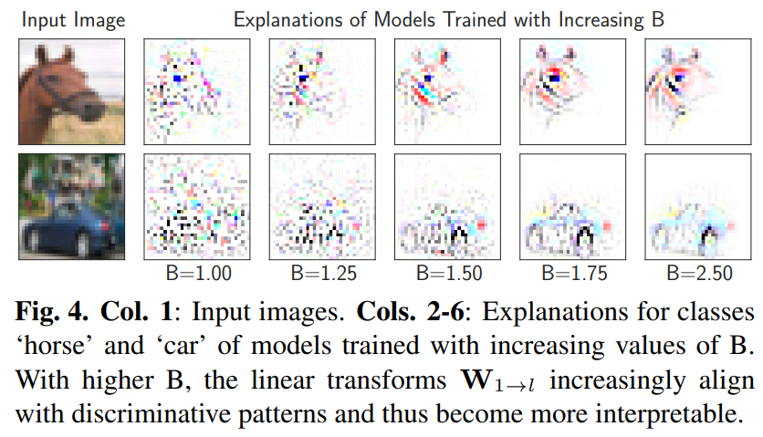
An increase in B affects the optimization of the model similar to the single unit case in Figure 2. For example, in Figure 4 we visualize [W1→l(xi)]yi for another sample i in the CIFAR-10 test set. As B is higher, the weight alignment increases noticeably from the piece-wise model (B=1) to the model with higher B (B=2.5). Importantly, we can quantify not only the visual quality of the explanation, but also the interpretability of the model. Especially, as shown in Figure 5, the spatial contribution maps defined as W1→l(xi) of the model with a larger value of B get much higher scores in the localization metric.
Advanced B-cos networks
- Classfication accuracies
Table 2 shows the classification accuracy of the pretrained model and the corresponding B-cos model. Except for the bottom row of Table 2, the rest were trained for 100 epochs with the Adam optimizer, 2.5e-4 learning rate, 256 batch size, and No weight decay. Also, the data was augmented with RandAugment. B-cos VGG 11 has a higher performance than the existing model. DenseNet-121 case can reduce the performance gap as shown in the last row of Table 2 through 200 epoch, 128 batch size, learning rate warm-up, and cosine learning rate schedule.
- Model interpretability
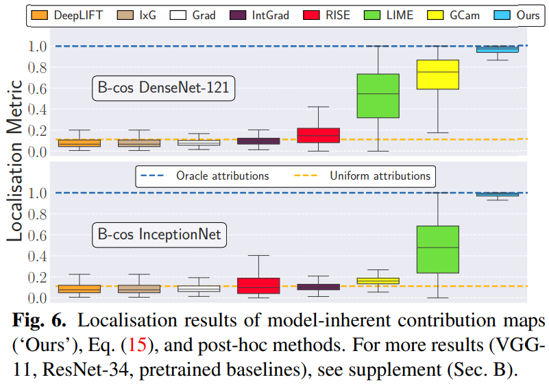
Figure 6 shows the explanation quality results evaluated by localization metrics for various post-hoc attribution methods as well as model-inherent contribution maps. In Table 2, the post-hoc method was evaluated in the existing pre-trained model and the corresponding B-cos model. In this paper, various gradient methods were evaluated (vanilla gradient (Grad), InputXGradient (IxG), Integrated Gradients (IntGrad), DeepLIFT, GradCam (GCam), perturbation-based methods (LIME, RISE)).As a result, the following two highlight the results: First, for all transformed B-cos architectures, the model-inherent explanation not only outperforms the post-hoc for model decision, but also approaches the optimal score in the localization metric. Second, the linear transformation (W1 For →l(x)) B-cos shows the interpretability of the model further improved.Qualitative evaluation of explanations
Every activation of the B-cos network is a result of the B-cos transform sequence. Therefore, every neuron n in layer I can be described by the corresponding linear transform [W1→l(x)]n.
For example, Figure 1 visualizes the linear transform of each class logit for various input images. During optimization, given alignment pressure, these linear transforms align with the class discriminant pattern of the input, so they actually resemble class entities.
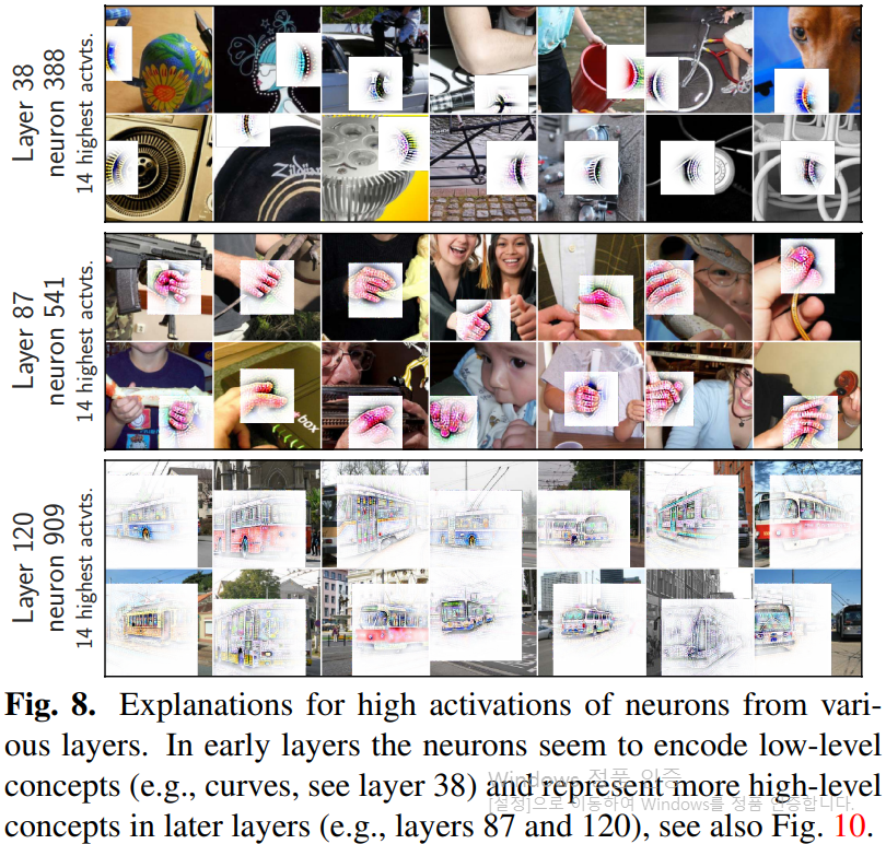
Similarly, Figures 8 and 10 visualize the description of the middle neuron. Specifically, Figure 8 shows descriptions of some of the most activated neurons for the validation set.
Figure 10 shows additional results for neurons in layer 87. The figure shows that some neurons are highly specific to certain concepts, such as the wheel (neuron 739), face (neuron 797), and eye (neuron 938). These neurons represent learning semantic concepts, rather than learning how to align to a simple, fixed pattern. Therefore, these are resistant to changes in color, size, and pose. In addition, several neurons strongly respond to watermarks in images, demonstrating the importance of DNN debugging. A watermark may not be meaningful, but it may be important depending on the task.
Finally, Figure 9 shows the descriptions of the model produce predictions with high uncertainty between the two most likely classes for images. Also, it shows the ∆ description that the difference between the contribution maps for the two classes. Through model-inherent linear mappings, W1→L, the model provides a human interpretable description of the uncertainty.
Limitation
The B-cos transform has computational overhead including the weights normalization and an additional down-scaling factor. this additional computation increases training and inference time by up to 60% compared to the baseline. However, this cost can be reduced in the future through the optimized implementation of the B-cos transform.
This work has integrated the B-cos transform with CNN. On the other hand, integrate B-cos into other types of architectures including recent work (vision) transformers is not be resolved.
Conclution
This study presented a new approach to giving deep neural networks a high level of inherent interpretability. B-cos transform was developed as a replacement for the linear transform to increase the weight-input alignment during the optimization process. and this paper was shown that this can greatly increase interpretability. This research shows that B-cos transform can faithfully reflect the underlying model. This is an important step in establishing confidence in DNN-based decisions.
Review
Summary
This paper described B-cos transform methods that improve the interpretability of the model by replacing linear and nonlinear functions such as ReLU through the weight-input alignment.Experiments showed improved interpretability while maintaining performance with a performance degradation of around 1% on commonly used architectures such as VGG-11, ResNet, DenseNet, and InceptionNet. In addition, by providing an explanation that can be interpreted by humans for the decision of the model with high uncertainty, it is possible to create a model that is more optimized for the task.
Strength
The strength of the B-cos transform is that it can be easily used as a replacement for linear functions including ReLU activation function. Assuming B = 1, it is the same as the existing model, and it can be easily optimized the interpretability by adjusting B. In addition, it has high interpretability while maintaining similar performance of the existing DNN architecture. Therefore, it is possible to increase the interpretability of various DNN architectures at low cost.
Weaknesses
As the limitation section of this paper says, the B-cos transform method can increase training and inference time by up to 60%. When using AI services or providing them to users, fast training and reasoning are important. In the case of super-large AI, which has had a great influence recently, a lot of costs are consumed in training and inference. At this time, an operation that increases cost may be very fatal to service provision.
Also, in this paper, add-ons to architectures such as ReLU, MaxPool, and skip connections are removed. These add-ons are affect model performances. In addition, this will be critical to application in other architectures mentioned in the paper. Therefore, it would be better to add a method to solve the mentioned add-on exclusion problem.
References
- [number in paper, number in blog]
[40, 1] C. Szegedy, V. Vanhoucke, S. Ioffe, J. Shlens, and Z. Wojna. Rethinking the Inception Architecture for Computer Vision. In Proceedings of the IEEE Conference on Computer Vision and Pattern Recognition (CVPR), 2016. 2, 5
[13, 2] Kaiming He, Xiangyu Zhang, Shaoqing Ren, and Jian Sun. Deep residual learning for image recognition. In Proceedings of the IEEE Conference on Computer Vision and Pattern Recognition (CVPR), 2016. 2, 5, 6
[35, 3] Karen Simonyan and Andrew Zisserman. Very Deep Convolutional Networks for Large-Scale Image Recognition. In Yoshua Bengio and Yann LeCun, editors, International Conference on Learning Representations (ICLR), 2015. 2, 5
[14, 4] Gao Huang, Zhuang Liu, Laurens Van Der Maaten, and Kilian Q Weinberger. Densely connected convolutional networks. In Proceedings of the IEEE Conference on Computer Vision and Pattern Recognition (CVPR), 2017
[12, 5] Ian Goodfellow, David Warde-Farley, Mehdi Mirza, Aaron Courville, and Yoshua Bengio. Maxout networks. In International Conference on Machine Learning (ICML), 2013.
[25, 6] Vinod Nair and Geoffrey E. Hinton. Rectified Linear Units Improve Restricted Boltzmann Machines. In International Conference on Machine Learning (ICML), 2010
[19, 7] Alex Krizhevsky. Learning multiple layers of features from tiny images. Technical report, University of Toronto, 2009. 2, 5.
[9, 8] Jia Deng, Wei Dong, Richard Socher, Li-Jia Li, Kai Li, and Li Fei-Fei. ImageNet: A large-scale hierarchical image database. In Proceedings of the IEEE Conference on Computer Vision and Pattern Recognition (CVPR), 2009
[26, 9] Adam Paszke, Sam Gross, Francisco Massa, Adam Lerer, James Bradbury, Gregory Chanan, Trevor Killeen, Zeming Lin, Natalia Gimelshein, Luca Antiga, Alban Desmaison, Andreas Kopf, Edward Yang, Zachary DeVito, Martin Raison, Alykhan Tejani, Sasank Chilamkurthy, Benoit Steiner, Lu Fang, Junjie Bai, and Soumith Chintala. PyTorch: An Imperative Style, High-Performance Deep Learning Library. In Advances in Neural Information Processing Systems (NeurIPS), 2019