[Python] Visualization

자주쓰는 matplotlib / seaborn

import matplotlib.pyplot as plt
import seaborn as sns


# print the graphs in the notebook
%matplotlib inline

# set seaborn style to white
sns.set_style("white")

boxplot(행, 열, 색상, 데이터)

sns.boxplot(x = "day", y = "total_bill", hue = "time", data = df);

df에서 & 연산자 사용법

df[(df['day']=='Thur') & (df['time'] == 'Dinner')]
#괄호 꼭 써라

histogram / FacetGrid

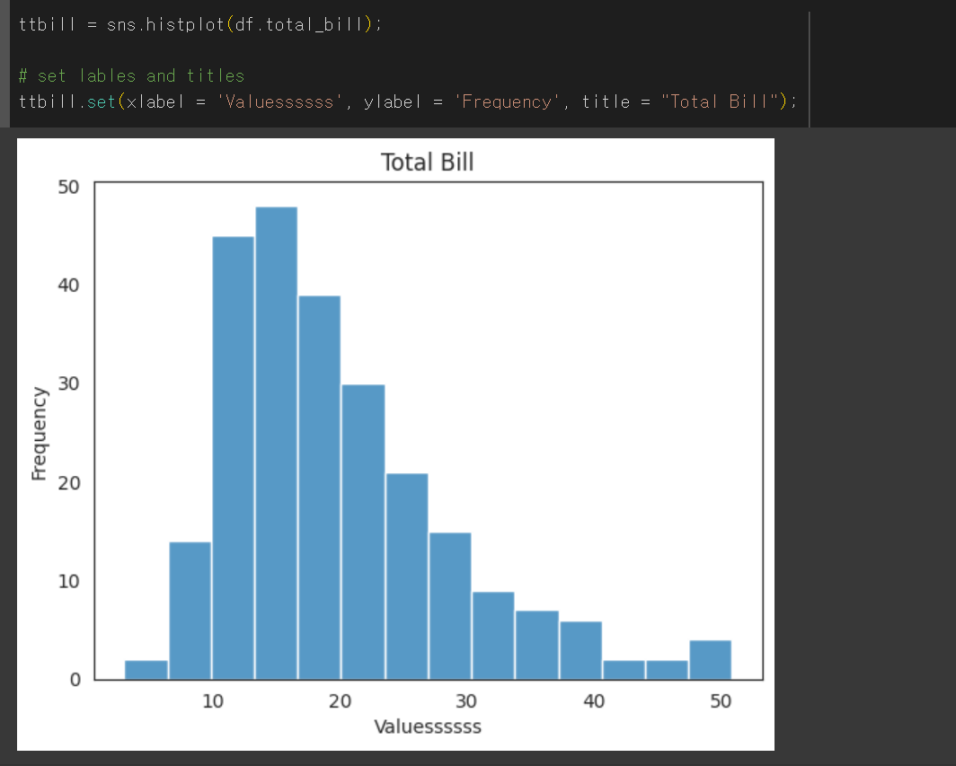
ttbill = sns.histplot(df.total_bill);

# set lables and titles
ttbill.set(xlabel = 'Value', ylabel = 'Frequency', title = "Total Bill");
# 여기선 x,y 아니고 xlabel ylabel임. histogram 지정하고 set 지정(단순이름 valuesssss로 바꿔봄)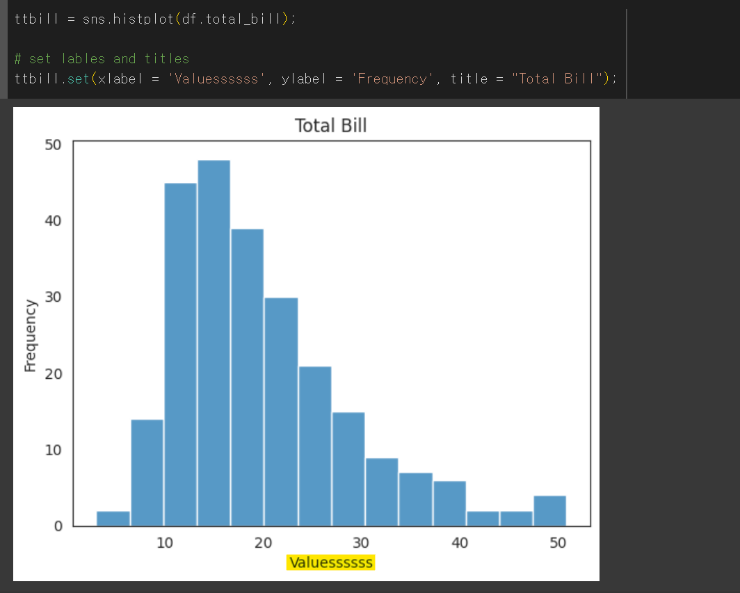

# better seaborn style
sns.set(style = "ticks")
plt.grid(True)
# creates FacetGrid
g = sns.FacetGrid(df, col = "time") #두개로 나눌 기준 col
g.map(plt.hist, "tip");  # tip 에 대해서 map

import numpy as np
# sort the values from the top to the least value and slice the first 5 items
df2 = df.Fare.sort_values(ascending = False)
# df3 = df.Fare

# create bins interval using numpy
binsVal = np.arange(0,600,10)
binsVal

# create the plot
plt.hist(df3, bins = binsVal)

# Set the title and labels
plt.xlabel('Fare')
plt.ylabel('Frequency')
plt.title('Fare Payed Histrogram')

# show the plot
plt.show()

scatter

g = sns.FacetGrid(df, col = "sex", hue = "smoker")
g.map(plt.scatter, "total_bill", "tip", alpha =.7) # alpha는 투명도

g.add_legend(); # 범례

pie chart

# sum the instances of males and females
males = (df['Sex'] == 'male').sum()
females = (df['Sex'] == 'female').sum()

# put them into a list called proportions
proportions = [males, females]

# Create a pie chart
plt.pie(
    # using proportions
    proportions,

    # with the labels being officer names
    labels = ['Males', 'Females'],

    # with no shadows
    shadow = False,

    # with colors
    colors = ['blue','yellow'],

    # with one slide exploded out
    explode = (0.15 , 0),           #벌어진 크기

    # with the start angle at 90%
    startangle = 90,                #시작 각도

    # with the percent listed as a fraction
    autopct = '%1.2f%%'
    )

# View the plot drop above
plt.axis('equal')

# Set labels
plt.title("Sex Proportion")

# View the plot
plt.tight_layout()
plt.show()

'%1.2f%%'는 문자열 포매팅을 의미합니다.
% : 문자열 포매팅을 시작하겠다는 표시입니다.
1.2f : 소수점 아래 두 자리까지 표시하겠다는 의미입니다.
%% : 실제 '%' 문자를 출력합니다. '%'를 출력하기 위해서는 '%%'와 같이 두 번 입력해야 합니다

lmplot

# creates the plot using
lm = sns.lmplot(x = 'Age', y = 'Fare', data = df, hue = 'Sex', fit_reg=False)

# set title
lm.set(title = 'Fare x Age')

# get the axes object and tweak it
axes = lm.axes
axes[0,0].set_ylim(-5,)           # y축 길이
axes[0,0].set_xlim(-5,85)         # x축 길이