sample project 의의

데이터 분석가도 머신러닝 딥러닝의 기초는 알아야 한다.
요건정의서가 매우 중요하다.
요건 정의서가 정확하지 않을 경우 진행하다가 방향을 잘못잡고 엎어지는 일이 많다.
분석가의 중요한 역량 중 하나
이 프로젝트를 진행했을 때 얻을 수 있는 효용 가치를 확인하는 사전 작업
매출 수요 예측 프로세스는 전처리를 이렇게하고 EDA를 하고 모델링을 이렇게 하는구나
이해하는 과정

프로젝트 순서

Process 01

데이터 살펴보기

고객마다 과거 진행한 캠페인(마케팅)에 대한 이력과, 현재 캠페인에서 수행된 데이터가 존재
duration은 예측시 제외 (※ 통화 시간에 따라 Y(가입여부) 결정되므로 제외)
데이터 명세 ⬇

데이터 전처리

수집된 데이터의 기본 정보들을 확인

(1) Data shape(형태) 확인

• df.shape()

(2) Data type 확인

• df.info()
  (3) Null값 확인 (※ 빈 값의 Data)
• df.isnull().sum()
  (4) Outlier 확인 (※ 정상적인 범주를 벗어난 Data)

pd.DataFrame(df.decribe()) 좋다

Duration 만 max값 및 표준편차가 이상적으로 컸다.

정기 예금 가입현황

df['y'].value_counts()

no 36548
yes 4640
4640 / (36548+4640) = 11%

범주형 변수 파악

# ▶ numerical, categorical data 나누기
numerical_list=[]
categorical_list=[]

for i in df.columns :
  if df[i].dtype == 'O' :
    categorical_list.append(i)
  else :
    numerical_list.append(i)

print("numerical_list :", numerical_list)
print("categorical_list :", categorical_list)

범주형과 수치형으로 column list를 생성

# ▶ numerical, categorical data 나누기
numerical_list=[]
categorical_list=[]

for i in df.columns :
  if df[i].dtype == 'O' :
    categorical_list.append(i)
  else :
    numerical_list.append(i)

print("numerical_list :", numerical_list)
print("categorical_list :", categorical_list)

numerical_list : ['age', 'duration', 'campaign', 'pdays', 'previous', 'emp.var.rate', 'cons.price.idx', 'cons.conf.idx', 'euribor3m', 'nr.employed']
categorical_list : ['job', 'marital', 'education', 'default', 'housing', 'loan', 'contact', 'month', 'day_of_week', 'poutcome', 'y']

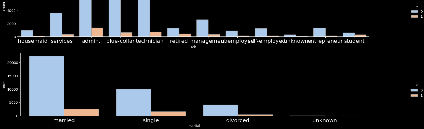
[직관 해석] catplot을 활용하여 Categorical 변수의 구성형태와 정기예금 가입 상황을 한눈에 살펴봄

import seaborn as sns
import matplotlib.pyplot as plt
%matplotlib inline
plt.style.use(['dark_background'])

for i in categorical_list :
  if i != 'y':
    sns.catplot(x=i, hue="y", kind="count",palette="pastel", edgecolor=".6",data=df);
    plt.gcf().set_size_inches(25, 3)
    plt.xticks(fontsize=16)

실행값

Process 02 Rule base 기반 상품 가입 예측

현업에서 경험적 지식에서 얻을 수 있는 노하우 기반
"이런 사람들의 가입률이 높겠구나" 하는 노하우, 데이터로 검증 후 적용

import numpy as np
df['y'] = np.where(df['y']=='yes', 1, 0)
df_job = df.groupby('job')['y'].agg(['count', 'sum'])
df_job['ratio'] = round((df_job['sum'] / df_job['count'])*100, 2)
df_job.sort_values(by=['ratio'], ascending = False)

현재 가입자['Y']를 값으로 하는 조건(여기서는 직관에 의해 JOB으로 설정)의 영향도를 확인해봄

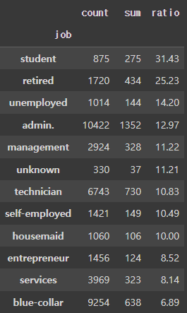
고객 Job(직업)에 따른 정기예금 가입률 비교

df_job=pd.DataFrame(df['y'].groupby(df['job']).value_counts())
df_job.columns=['cnt']
df_job=df_job.reset_index()
df_job.head(5)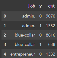

pivot table을 활용하여 하나의 row로 변환

df_job = pd.pivot_table(df_job,        # 피벗할 데이터프레임
                     index = 'job',    # 행 위치에 들어갈 열
                     columns = 'y',    # 열 위치에 들어갈 열
                     values = 'cnt')   # 데이터로 사용할 열

df_job = df_job.reset_index()
df_job.head(5)

# 가입률(sign_ratio) 추가
df_job['sign_ratio'] =   round((df_job['yes'] / (df_job['yes'] + df_job['no'])) * 100,1)
df_job.sort_values(by=['sign_ratio'], ascending =False)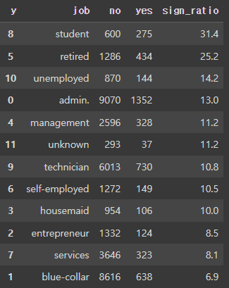

Student(학생)의 가입률이 가장 높고, 뒤이어 은퇴 고객의 가입률이 높음 (※ 평균가입률 11%)

내림차순 정렬해봄

import seaborn as sns
import matplotlib.pyplot as plt
%matplotlib inline
plt.style.use(['dark_background'])
order = df_job.groupby('job')['sign_ratio'].sum().sort_values(ascending =False).index

avg_ratio = round((df_job['yes'].sum() / (df_job['yes'].sum() + df_job['no'].sum())) * 100,1)
print(avg_ratio)

g = sns.catplot(x="job", y="sign_ratio", kind='bar', palette="ch:.25", data=df_job, order=order);
g.ax.axhline(11.3, ls='--', color='r', label = 'average')

plt.rc('xtick', labelsize=10)
plt.gcf().set_size_inches(25, 5)
g.ax.legend()
plt.show()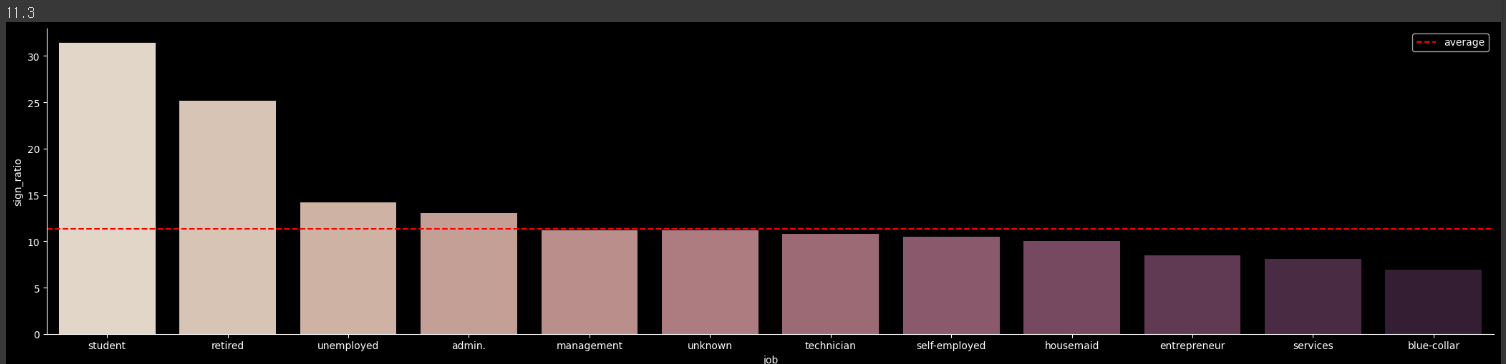

Categorical(범주형) 변수에 대해서 가입률 비교를 모두 진행

▶ Feature별 가입률이 가장 높은 Row에 대해서만 출력

for i in categorical_list :
  # 1단계
  df_job=pd.DataFrame(df['y'].groupby(df[i]).value_counts())
  df_job.columns=['cnt']
  df_job=df_job.reset_index()

  # 2단계
  df_job = pd.pivot_table(df_job,        # 피벗할 데이터프레임
                      index = i,         # 행 위치에 들어갈 열
                      columns = 'y',     # 열 위치에 들어갈 열
                      values = 'cnt')    # 데이터로 사용할 열

  # 3단계
  df_job = df_job.reset_index()

  # 4단계
  df_job['sign_ratio'] =   round((df_job['yes'] / (df_job['yes'] + df_job['no'])) * 100,1)

  df_job=df_job.sort_values(by=['sign_ratio'], ascending=False)

  print(df_job.iloc[0:1,:])
  print('')

▶ 상위에서 평균 가입률(11%) 대비 높았던 조건을 OR조건으로 새로운 Rule(규칙)을 정의

df_rule = df[ (df['job'] == 'student') |
# (df['marital'] == 'unknown') |
# (df['education'] == 'illiterate') |
# (df['default'] == 'no') |
# (df['housing'] == 'yes') |
# (df['loan'] == 'no') |
(df['contact'] == 'cellular') |
(df['month'] == 'mar') |
# (df['day_of_week'] == 'thu') |
(df['poutcome'] == 'success') ]
a= df_rule['y'].value_counts()['no']
b= df_rule['y'].value_counts()['yes']
b/(a+b)

▶ Rule에 의한 타겟 고객군을 추출 했을 때 평균 14% 가입률을 보임
14.9448%

Process 03 ML활용 상품 가입 예측

모델링을 수행하기 위해 Feature와 예측값인 Y로 데이터를 나눔
학습과 예측을 위한 train/test set 분할
But, Train/Test set에는 문자(str) 형태 데이터를 input 할 수 없음
Model 에서 이해할 수 있는 1,0으로 변경 > encoding

import numpy as np
df['y']=np.where(df['y']=='yes', 1, 0)

모델링 데이터 전처리

▶ 모델링을 학습하기 위한 Feature(X)와 Y데이터를 구분하는 단계

from sklearn.model_selection import train_test_split
from sklearn.ensemble import RandomForestClassifier
from sklearn import metrics

X=df.drop(['duration','y'], axis=1)
Y=df['y']

x_train, x_test, y_train, y_test = train_test_split(X, Y, test_size=0.3, stratify=Y)

print(x_train.shape)
print(y_train.shape)

print(x_test.shape)
print(y_test.shape)

결과값
(28831, 19)
(28831,)
(12357, 19)
(12357,)

for i in categorical_list :
  print(i, df[i].nunique())

범주형 변수들의 문자 -> 숫자화

▶ Categorical(범주형) 변수는 One-hot-encoding or Label-encoding을 통해 숫자형 변수로 변경해야함

▶ One-hot-encoding은 차원이 많은 변수에는 불리, Label-encoding은 회귀관련 알고리즘에서는 사용 어려움.(※Tree 계열 알고리즘에서는 사용 가능)

from sklearn.preprocessing import LabelEncoder

for col in categorical_list:
    le = LabelEncoder()
    x_train[col] = le.fit_transform(x_train[col])
    x_test[col] = le.transform(x_test[col])

x_train[categorical_list].head()

테스트 데이터를 변환할 때는 학습 데이터에서 학습한 인코더를 그대로 사용해야 한다는 것입니다. 따라서 x_test에는 fit_transform 대신 transform을 사용하였습니다.

모델 학습 및 평가

▶ 학습

from sklearn.metrics import classification_report
rfc = RandomForestClassifier(random_state=123456)
rfc.fit(x_train, y_train)

▶ 예측

y_pred_train = rfc.predict(x_train)
y_pred_test = rfc.predict(x_test)

print(classification_report(y_train, y_pred_train))
print(classification_report(y_test, y_pred_test))

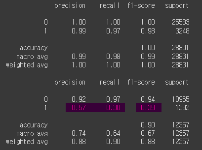
재현율이 30% test에 적합하지 않은 것으로 판단된다.
학습데이터에 과적합되었다 -> 그래서 초매개변수 수정

Hyper parameter 튜닝

모델 성능을 올리기 위한 옵션 조절

▶ RandomForestClassifier 객체 생성 후 GridSearchCV 수행

from sklearn.model_selection import GridSearchCV

params = { 'n_estimators' : [400],
           'max_depth' : [6, 8, 10]
            }


rf_clf = RandomForestClassifier(random_state = 12345, n_jobs = -1)
grid_cv = GridSearchCV(rf_clf, param_grid = params, cv = 3, n_jobs = -1, scoring='precision')
grid_cv.fit(x_train, y_train)

print('최적 하이퍼 파라미터: ', grid_cv.best_params_)
print('최고 예측 정확도: {:.4f}'.format(grid_cv.best_score_))

최적 하이퍼 파라미터: {'max_depth': 6, 'n_estimators': 500}
최고 예측 정확도: 0.7025

▶ Best score 기준 재학습

rfc = RandomForestClassifier(n_estimators=400, max_depth=6, random_state = 123456)
rfc.fit(x_train, y_train)

y_pred_train = rfc.predict(x_train)
y_pred_test = rfc.predict(x_test)

print(classification_report(y_train, y_pred_train))
print(classification_report(y_test, y_pred_test))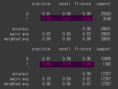

f1 - score가 너무 떨어졌는데, test set과 유사한 수준으로 맞추는게 더 의미가 있다고함.

중요 변수 파악

Feature IMP 분석을 통한 중요변수 파악

import matplotlib.pyplot as plt
import seaborn as sns
%matplotlib inline
plt.style.use(['dark_background'])

ftr_importances_values = rfc.feature_importances_
ftr_importances = pd.Series(ftr_importances_values, index = x_train.columns)
ftr_top20 = ftr_importances.sort_values(ascending=False)[:20]

plt.figure(figsize=(8,6))
plt.title('Feature Importances')
sns.barplot(x=ftr_top20, y=ftr_top20.index)
plt.show()

# ▶ 1위 변수 탐색
sns.distplot(df['age']);   ## nr.employer 대신 넣어봄
plt.gcf().set_size_inches(5 ,5)


# ▶ 구간화  <<< age로 진행함
import numpy as np
# df['nr.employed_gp'] = np.where (df['nr.employed'] <= 5000, '5000 이하',
#                            np.where(df['nr.employed'] <= 5200, '5000~5200', '5200 초과'))

df['age'] = np.where(df['age'] <= 19, '10대',
                     np.where(df['age'] <= 29, '20대',
                     np.where(df['age'] <= 39, '30대',
                     np.where(df['age'] <= 49, '40대',
                     np.where(df['age'] <= 59, '50대',
                     np.where(df['age'] <= 69, '60대',
                     np.where(df['age'] <= 79, '70대', '80대 이상')))))))

# # ▶ 평가
# df_gp = df.groupby('nr.employed_gp')['y'].agg(['count', 'sum'])
# df_gp['ratio'] = round((df_gp['sum'] / df_gp['count']) * 100, 1)
# df_gp

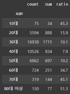
df_gp = df.groupby('age')['y'].agg(['count', 'sum'])
df_gp['ratio'] = round((df_gp['sum'] / df_gp['count']) * 100, 1)
df_gp

저장 및 불러오기

import pickle
# 모델 저장
saved_model = pickle.dumps(rfc)

# 모델 Read
clf_from_pickle = pickle.loads(saved_model)

결론

유의미한 결과를 얻기 어려운 분석이라고 판단된다.
nr.employer 는 판매직원 은행의 직원수라고 추정됨.
=기업, 조직, 또는 경제 전체의 직원 수를 분기별로 나타내는 수치 지표를 의미
고객 정보보다 외부 변수(nr.number, 유리보 3개월금리, 실업율, cpi 등) 에 영향을 많이 받는 것 같음. 이 분석 결과로는 고객 정보에 대한 내용은 없고 "nr.number가 높은 시기에 마케팅을 해야한다." 정도의 결과가 나오는 것 같다. 그래서 시작부터 외부 변수와 고객 변수를 나눠서 수행해야했지 않나 생각
현재는 모든 변수를 하나로 묶어서 진행한 것 같은데, 아래와 같이 두가지 분석 목표를 가지고 설계하는 것은 어떤지 궁금해졌다.

현 분석 목표 : 모든 변수를 포함하여 고객 가입률에 영향을 미치는 변수 찾기

변경 1. 분석 목표 : 가입할 가능성이 높은 고객의 성향 찾기
고객에 대한 변수만을 모아서 수행
poutcome, month, age, job과 같은 고객에게 매칭되는 정보로만 진행

변경 2. 분석 목표 : 외부 변수로 인한 가입률 높은 "시기" 추출 + 이 시기에 가입률 높은 "고객 변수" 추출

멘토님은 변경 1안은 큰 의미 없어 보이고, 현 목표와 변경 2안을 진행해서 더 좋은 분석을 뽑아 보라고 함