2. Find two images and compute their corresponding spectrum and
phase angle, then visualize them. Synthesis new images using one
image’s spectrum and another image’s phase angle, visualize them.
( 30 points)
위상각,스펙트럼 푸리에변환이 쓰이는 예제이다.
이 문제를 풀기전에 기본적으로 영상과 푸리에에 관한 관계가 어떤건지에 대해 먼저 분석 해보고 시작하자.
푸리에 급수란 모든 주기함수는 각기 다른 주파수의 사인과 코사인 함수에 각기 다른 계수를 곱한 합으로 표현할 수 있음을 나타낸 것이다.
푸리에 변환이란 주기적이지 않은 함수들도 가중 함수로 곱해진 싸인과 코싸인들의 적분으로 표현될 수 있음을 나타낸 것이다.
이를 다른 말로 표현 하자면 시간 영역을 푸리에 변환 시키면 주파수 영역으로 표현할 수 있는 것인데 이 주파수 영역에 각 주파수의 성분의 위상 정보가 들어있다.

근데 여기서 의문이 생긴다. 도대체 푸리에 급수를 왜 쓰는걸까?
가장 큰 이유는 우리가 구해야 하는 함수 f(t)의 해석이 거의 불가능 하기 때문이다.
f(t)라는 함수를 사용 하는것과 삼각함수의 무한급수를 사용 하는것 중 f(t)를 그대로 사용하는게 낫지 않냐 생각할 수 있으나
f(t)에 대해 아는것이 없으니 이를 급수로 사용해 해석하여 표현하는 것이다.
그럼 시간함수를 푸리에 변환해서 주파수 영역에서 쓰는 이유는 뭘까?
이유는 주파수 영역에서의 사용이 더 쉽기 때문이다. 신호파형이 계속해서 변하는데 시간영역으로 해석하는것은 비효율적이다.
푸리에 급수와 푸리에 변환이 왜 영상에서 쓰이는지 당장은 잘 이해가 가지 않는다, 이 과목의 이름이 왜 '디지털 영상 처리' 인지 먼저 확실하게 이해를 해야 할 것 같다.
정확히 말하자면 시간 영역이 아닌, 공간 영역이라는 단어가 확실하게 이해가 되지 않는다고 해야할까?
먼저 생각한것은 시간 영역에서의 푸리에 변환은 시간과 그에 따른 강도의 변화에 대한 그래프를 주파수 영역으로 표현 한 것이다.
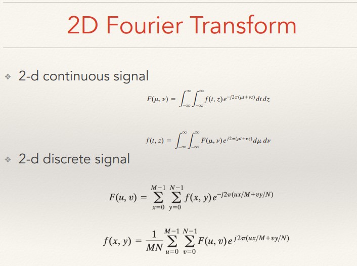
이번 장에 나오는 내용들을 보면 유독 2D 푸리에 변환에 대한 설명이 많고 그것을 강요 하던데 그렇다면 이렇게 생각하면 어떨까?
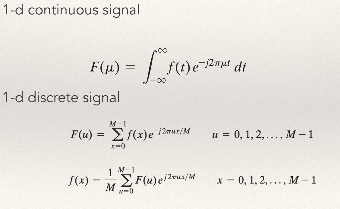
우리가 수업시간에 배운 1D 푸리에 변환은 기본적으로 DSP 에서 보던 푸리에 변환과 그 유형이 같다.
우리는 차원이라는 개념을 설명할 때 보통 1차원은 선, 2차원은 면, 3차원은 공간이라 한다.
선을 적분해서 쌓아주면 면, 면을 적분해서 쌓아주면 공간...
감이 좀 잡힌것 같다. 헷갈릴 수 있으니 지금부터 이미지의 가로, 세로축을 라고 하고 주파수 도메인을 라고 표현 하겠다.
그럼 만약에 우리가 512 x 512 의 이미지가 있다고 한다면 x 축을 픽셀 좌표 각 픽셀당 밝기를 f(x) 라고 생각하고 1줄로 쭉 나열하면 길이가 512 인 비주기 신호가 완성 될 것이다.
그리고 이렇게 적분한 1차원 푸리에 변환을 y축만큼 다시 쌓아주는것이다.
그럼 결과적으로 가로 세로로 각각 u 와 v의 주파수 도메인을 가지고 있는 푸리에 변환된 함수가 탄생한다.
근데 이걸 왜쓸까? 푸리에 변환을 했을때 무언가 이득이 있나?
푸리에 변환을 하는 주된 이유는 연산의 편리함에 있다. 예를들어 가우스 필터를 이용한 회선(컨벌루션) 연산으로 영상 잡음을 제거할 때 공간 영역에서
가우스 필터의 마스크 크기가 증가할수록 연산 시간또한 마스크 면적에 비례해 증가하는데
주파수 영역으로 변환된 신호에서 회선 연산은 주파수 성분 사이의 곱셈 연산으로 수행되 마스크의 크기에 상관 없이 연산 시간이 일정하게 유지된다.
또한 영상을 주파수 영역으로 변환하게 되면 영상의 메모리 용량을 줄이는 압축 작업도 할 수 있다.
위에서 주파수 영역으로 변환한 그래프를 보면 영상의 대부분이 저주파 성분으로 되어 있다. 따라서 미미하게 존재하는 고주파 성분을 영상 저장 과정에서 생력하면 시각적으로 식별할 수 있는 영상의 품질 저하를 최소화하면서 저장에 사용하는 메모리 용량도 최소화 할 수 있다. 이렇게 영상의 일부 성분을 제거하여 압축하는 것을 손실 압축이라고 하는데 주파수 영역 변환을 이용한 방법은 손실되는 정보에 비하여 메모리 용량 감소가 뛰어나다는 장점이 있다.
파이썬에는 물론 fft dft가 모두 구현 되있다. 이대로 문제를 풀어도 되긴 하는데 어차피 DSP 실험도 있고 시간 영역 주파수 영역에 고통받는 나 자신을 위해 DFT부터 FFT까지 간단하게 구현 해보겠다.
그 전에 간단한 시간영역의 그래프를 그려보자.
import cv2
import numpy as np
import matplotlib.pyplot as plt
"""
newly knowed knowledge
np.linespace(start,end,n) : Divide the start and end points by n intervals.

"""
x = np.linspace(0, 20, 201) #0~20을 201개 구간(0.1)로 나눕니다.
y = np.sin(x)

plt.figure(figsize = (6, 4))
plt.plot(x, y, 'b') #Floating sin graph
plt.ylabel('Amplitude')
plt.xlabel('Location (x)')
plt.show()

fig = plt.figure(figsize = (8,6))
times = np.arange(5)#0~4 범위의 정수 생성
print(times)
n = len(times)

for t in times:
    plt.subplot(n, 1, t+1)
    y = np.sin(x + 2*t)
    plt.plot(x, y, 'b')
    plt.plot(x[25], y [25], 'ro')# x=2.5, y=sin(x=2.5)
    plt.ylim(-1.1, 1.1)
    plt.ylabel('y')
    plt.title(f't = {2*t}')

plt.xlabel('location (x)')
plt.tight_layout()
plt.show()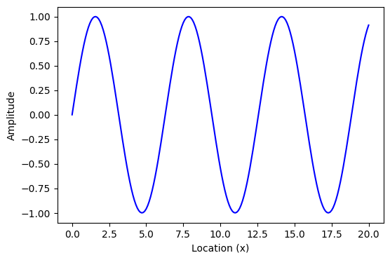
[0 1 2 3 4]
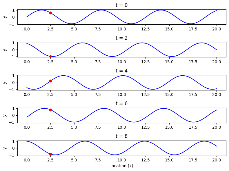
파동그래프에 대해 간단하게 그려보았다. 시간영역에서의 진폭, 위상으로 파동을 구현 해봤으니 이걸 이제 복잡한 파동, 더 나아가 공간 영역에서 사용할 수 있게 만들어 보자!
DFT(이산 푸리에 변환)
이산 푸리에 변환은 시간 영역의 신호에 오일러 방정식을 곱해 주파수 영역으로 변환 시켜준다고 생각하면 된다.
N = 샘플 수
n = 현재 샘플
k = 현재 주파수, 여기서k∈[0,N−1]
= 샘플 n에서의 사인 값
= 진폭과 위상의 정보를 모두 포함하는 DFT
일단 비주기 신호를 하나 만들어서 DFT 공식을 적용시킬 수 있나 해보자
주파수가 1Hz, 4Hz, 7Hz이고 진폭이 3, 1, 0.5이고 위상이 모두 0인 3개의 사인파를 생성해보자.
조건은 0~1 구간으로 100개 구간으로 샘플링 후
  # sampling rate
sr = 128
# sampling interval
ts = 1.0/sr
t = np.arange(0,1,ts)

freq = 1.
x = 3*np.sin(2*np.pi*freq*t)

freq = 4
x += np.sin(2*np.pi*freq*t)

freq = 7
x += 0.5* np.sin(2*np.pi*freq*t)

plt.figure(figsize = (8, 6))
plt.plot(t, x, 'r')
plt.ylabel('Amplitude')

plt.show()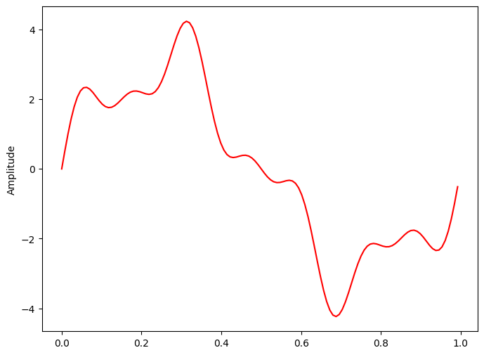
def DFT(x):

  N = len(x)# period(every interval) of x
  n = np.arange(N)
  k = n.reshape((N, 1))
  W = np.exp(-2j * np.pi * k * n / N)

  X = np.dot(W, x)#convolutuon of vector e

  return X
"""
stem(x,y,use_line_collection = True)

stemlines.set_visible(False) ## stem line 안보이게
baseline.set_visible(False) ## base line 안보이게
markers.set_color('red')# 색상 고를 수 있게
stemlines.set_linestyle('--') #라인 스타일 바꿀 수 있게
stemlines.set_color('purple') #라인 색깔 바꿀 수 있게 해줌
"""

X = DFT(x)
# calculate the frequency
# sampling rate is 100 and interval is 0.01

N = len(X)
n = np.arange(N)
print("lenth of N: ",N)
print("component of N: ",n)

T = N/sr #because function is unperiodic, we can guess T equals to 1
freq = n/T #frequency is 100

plt.figure(figsize = (8, 4))
plt.stem(freq, abs(X), 'b', \
       markerfmt=" ", basefmt="-b")
plt.xlabel('Freq (Hz)')
plt.ylabel('DFT Amplitude |X(freq)|')
plt.show()
lenth of N: 128
component of N: [ 0 1 2 3 4 5 6 7 8 9 10 11 12 13 14 15 16 17
18 19 20 21 22 23 24 25 26 27 28 29 30 31 32 33 34 35
36 37 38 39 40 41 42 43 44 45 46 47 48 49 50 51 52 53
54 55 56 57 58 59 60 61 62 63 64 65 66 67 68 69 70 71
72 73 74 75 76 77 78 79 80 81 82 83 84 85 86 87 88 89
90 91 92 93 94 95 96 97 98 99 100 101 102 103 104 105 106 107
108 109 110 111 112 113 114 115 116 117 118 119 120 121 122 123 124 125
126 127]
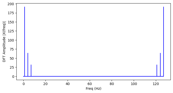
여기에서 DFT의 출력이 샘플링 속도의 절반에서 대칭임을 알 수 있는데, 샘플링 속도의 이 절반을 나이퀴스트 주파수 또는 폴딩 주파수라고 한다.
이는 샘플링 주파수의 절반 미만인 주파수 성분만 포함하는 경우 속도로 샘플링된 신호가 완전히 재구성될 수 있으므로 DFT의 최고 주파수 출력은 샘플링 속도의 절반이라는 것이다.
n_oneside = N//2
# get the one side frequency
f_oneside = freq[:n_oneside]

# normalize the amplitude
X_oneside =X[:n_oneside]/n_oneside

plt.figure(figsize = (8, 4))
plt.subplot(121)
plt.stem(f_oneside, abs(X_oneside), 'b', \
       markerfmt=" ", basefmt="-b")
plt.xlabel('Freq (Hz)')
plt.ylabel('DFT Amplitude |X(freq)|')

plt.subplot(122)
plt.stem(f_oneside, abs(X_oneside), 'b', \
       markerfmt=" ", basefmt="-b")
plt.xlabel('Freq (Hz)')
plt.xlim(0, 10)
plt.tight_layout()
plt.show() 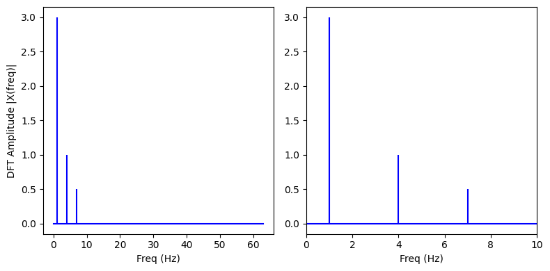
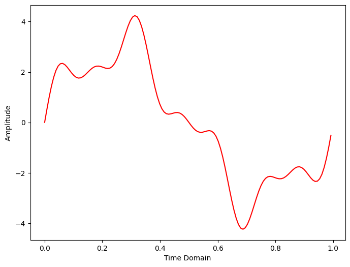
Inverse DFT는 주파수 영역의 시간 영역 변환이고
공식은 다음과 같이 적용하면 된다.
def IDFT(X):

  N = len(X)# period(every interval) of x
  n = np.arange(N)
  k = n.reshape((N, 1))
  W_ = np.exp(2j * np.pi * k * n / N)

  x = 1/N*(np.dot(W_, X))#convolutuon of vector e

  return x
x_IDFT = IDFT(X)
plt.figure(figsize = (8, 6))
plt.plot(t, x_IDFT, 'r')
plt.xlabel('Time Domain')
plt.ylabel('Amplitude')

plt.show()
c:\Users\joong\anaconda3\envs\ml\lib\site-packages\matplotlib\cbook__init__.py:1369: ComplexWarning: Casting complex values to real discards the imaginary part
return np.asarray(x, float)
Fast fourier transform(FFT)
고속 푸리에 변환(FFT)은 시퀀스의 DFT를 계산하는 효율적인 알고리즘이다.
DFT를 더 작은 DFT로 재귀적으로 분할하여 계산을 중단시키는 분할 정복 알고리즘인데
DFT의 복잡성을 O(n2)에서 O(nlogn)로 감소시킨다. 여기서 n은 데이터의 크기이다.
DFT의 대칭
FFT는 DFT의 대칭성을 이용하는 알고리즘인데 무슨 말인지 알아보자.
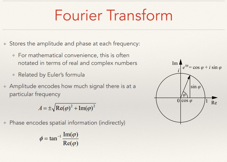
기본적으로 우리는 푸리에 변환이 오일러 방정식을 기본으로 구현하는것을 알고있고 오일러 방정식이 실수와 허수축을 기준으로 원형으로 회전 하는 특성을 알고 있다.
여기서 주어진 이산 신호를 여러 개의 길이가 짧은 신호로 분할하여 분할된 신호들의 DFT를 구한 뒤, 그 결과들을 결합해서 주어진 신호의 DFT를 수행하는것이 기본적인 로직이다.
구현 방법으로는 우선 전체 시리즈를 짝수와 홀수로 나눠주고 이것이 대칭임을 이용해서 재귀적으로 계속해서 분할 해준다. 이렇게 반복하다보면 최종적으로 계산량이 많이 줄어든다.
이제 FFT를 구현해보자.
def FFT(x):
  N = len(x)

  if N == 1:
      return x
  else:
      X_even = FFT(x[::2])
      X_odd = FFT(x[1::2])
      W = np.exp(-2j*np.pi*np.arange(N)/ N)

      X = np.concatenate(\
          [X_even+W[:int(N/2)]*X_odd,
           X_even+W[int(N/2):]*X_odd])
      return X
X=FFT(x)

# calculate the frequency
N = len(X)
n = np.arange(N)
T = N/sr
freq = n/T

plt.figure(figsize = (8, 4))
plt.subplot(121)
plt.stem(freq, abs(X), 'b', \
       markerfmt=" ", basefmt="-b")
plt.xlabel('Freq (Hz)')
plt.ylabel('FFT Amplitude |X(freq)|')

# Get the one-sided specturm
n_oneside = N//2
# get the one side frequency
f_oneside = freq[:n_oneside]

# normalize the amplitude
X_oneside =X[:n_oneside]/n_oneside

plt.subplot(122)
plt.stem(f_oneside, abs(X_oneside), 'b', \
       markerfmt=" ", basefmt="-b")
plt.xlabel('Freq (Hz)')
plt.ylabel('Normalized FFT Amplitude |X(freq)|')
plt.tight_layout()
plt.show() 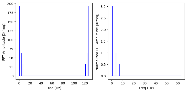
def IFFT(X):
  N = len(X)

  if N == 1:
      return X
  else:
      x_even = IFFT(X[::2])
      x_odd = IFFT(X[1::2])
      W_ = np.exp(2j*np.pi*np.arange(N)/ N)

      x = (np.concatenate([x_even+W_[:int(N/2)]*x_odd, x_even+W_[int(N/2):]*x_odd]))
      return (1/2) * x
print(len(X))
x_IFFT = IFFT(X)
plt.figure(figsize = (8, 6))
plt.plot(t, x_IFFT, 'r')
plt.xlabel('Time Domain')
plt.ylabel('Amplitude')

plt.show()
128

def FFT(x):
x = np.asarray(x, dtype=complex)
N = len(x)
if N == 1:
return x
else:
X_even = FFT(x[::2])
X_odd = FFT(x[1::2])
W = np.exp(-2j*np.pi*np.arange(N)/ N)
X = np.concatenate([X_even+W[:int(N/2)]*X_odd,X_even+W[int(N/2):]*X_odd])#Seperate and calculate the function, It's pretty similar logic with merge sort
return X
def IFFT(X):
N = len(X)
if N == 1:
return X
else:
x_even = IFFT(X[::2])
x_odd = IFFT(X[1::2])
W_ = np.exp(2j*np.pi*np.arange(N)/ N)
x = (np.concatenate([x_even+W_[:int(N/2)]*x_odd, x_even+W_[int(N/2):]*x_odd]))#concatenate X_k,X_k+N
return (1/2) * x
def FFT2D(x):
"""
Let's think how to implement the 2D FFT
There's 512 x 512 2D image array
at first, take 512(column) fouruier transformed list,
Then, We can get the 512 1D array of fourier transformed list
we Know space signal have x and y coordinate, should take fourier transform in every columns once more
"""
height, width = x.shape[0], x.shape[1]
#X =np.zeros(x.shape)
X =np.zeros(x.shape,dtype=complex)
if len(X.shape) == 2:
for i in range(height):
X[i, :] = FFT(x[i, :])
#print(X[:3])
for i in range(width):
X[:, i] = FFT(X[:, i])
#print(X[:3])
return X
def IFFT2D(X):
height, width = X.shape[0], X.shape[1]
x =np.zeros(X.shape,dtype=complex)
#X =np.zeros(x.shape)
if len(X.shape) == 2:
for i in range(height):
x[i, :] = IFFT(X[i, :])
for i in range(width):
x[:, i] = IFFT(x[:, i])
x=np.real(x) #Image data of dtype complex128 cannot be converted to float
return x
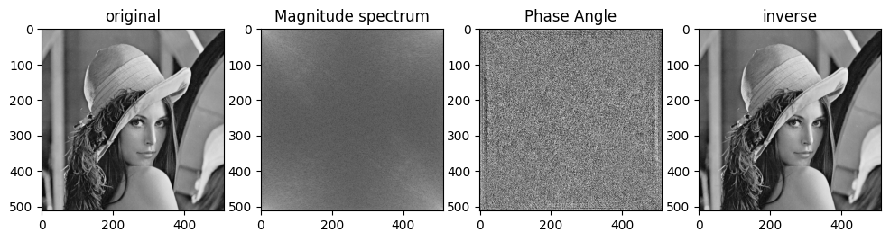
img = cv2.imread('../Lenna.png')
gray = cv2.cvtColor(img, cv2.COLOR_BGR2GRAY)#take grayscale
height, width = gray.shape
dimension = np.zeros(gray.shape, dtype=complex)
print(height,width)
dft = FFT2D(gray)
out = np.log(1+np.abs(dft))
inverse_dft = IFFT2D(dft)
#out2 = 20*np.log(np.abs(inverse_dft))
fig = plt.figure(figsize=(12,8))
plt.subplot(141),plt.imshow(gray, cmap='gray'),plt.title('original')
plt.subplot(142),plt.imshow(out, cmap='gray'),plt.title('Magnitude spectrum')
plt.subplot(143), plt.imshow(np.angle(dft), "gray"), plt.title("Phase Angle")
plt.subplot(144),plt.imshow(inverse_dft, cmap='gray'),plt.title('inverse')
plt.show()512 512
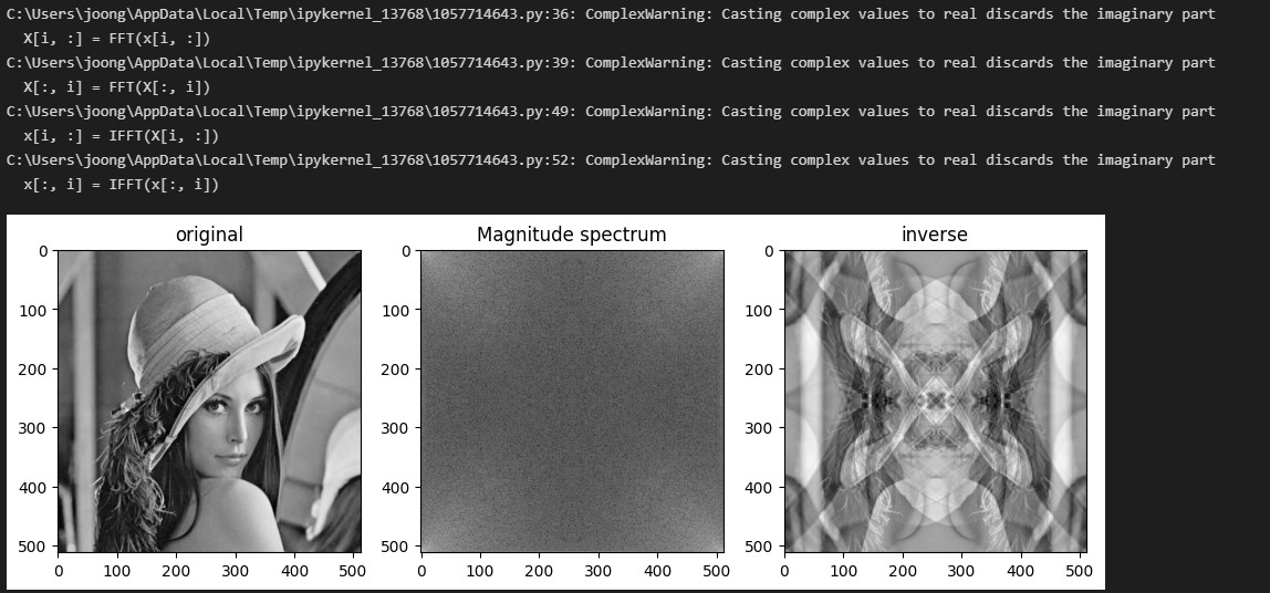
fast fft를 사용했는데도 함수 실행이 10초 가까이 걸린다.
참고로 이미지를 실수축으로만 실행하면 상당히 재미있는 결과가 나온다.
파이썬에 내장되있는 fft함수를 써서 위상을 표시하고 비교 해보겠다.
""" Logic
First, Let's implement every function through opencv and see the result
after than, I will implement fourier transform and compare result.
"""
def fourier(source):
  img = cv2.imread(source)
  gray = cv2.cvtColor(img, cv2.COLOR_BGR2GRAY)#take grayscale

  img_c1 = gray
  img_c2 = np.fft.fft2(img_c1)
  img_c3 = np.fft.fftshift(img_c2)
  img_c4 = np.fft.ifftshift(img_c3)
  img_c5 = np.fft.ifft2(img_c4)

  fig=plt.figure(figsize=(20,12))
  plt.subplot(161), plt.imshow(img_c1, "gray"), plt.title("Original Image")
  plt.subplot(162), plt.imshow(np.log(1+np.abs(img_c2)), "gray"), plt.title("Magnitude Spectrum")
  plt.subplot(163), plt.imshow(np.log(1+np.abs(img_c3)), "gray"), plt.title("Centered Spectrum")
  plt.subplot(164), plt.imshow(np.angle(img_c2), "gray"), plt.title("Phase Angle")
  plt.subplot(165), plt.imshow(np.log(1+np.abs(img_c4)), "gray"), plt.title("Decentralized")
  plt.subplot(166), plt.imshow(np.abs(img_c5), "gray"), plt.title("Processed Image")

  plt.show()
fourier('../Lenna.png') 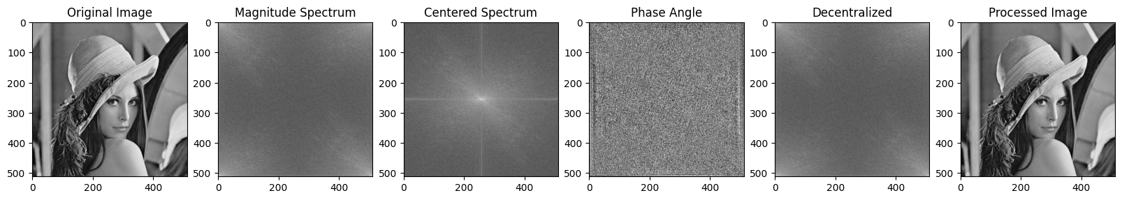
fourier('../Cameraman.png') 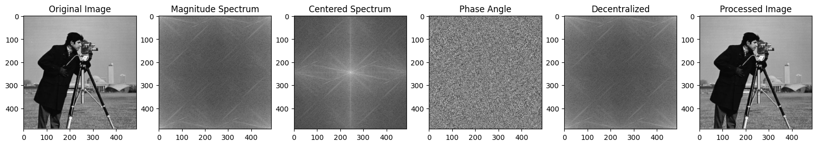
reference:
https://everyday-image-processing.tistory.com/165
https://1coding.tistory.com/139#%EB%--%--%EC%A-%--%ED%--%B-%--%EC%--%--%EC%--%--%EC%-D%--%--%EB%B-%--%ED%--%--%--%EA%B-%BC%EC%A-%--%---%EB%-B%A-%EA%B-%--%---%--%EB%B-%--%ED%--%B-%ED%--%--
https://pythonnumericalmethods.berkeley.edu/notebooks/chapter24.02-Discrete-Fourier-Transform.html
ppt