1.
static, dynamic data
static data refers to known parameters such as processing time or due date.
start or completion times as examples of dynamic data that arise from the actual schedule.
Schedule robustness
refers to the
- ability of a schedule to maintain acceptable performance despite disruptions.
- One technique to increase robustness is to include buffer time or reserve capacity, which helps absorb small delays without needing to fully reschedule.
The scheduling model aimed at
- maximizing throughput in a production system with automated material handling is often related to
- Just-In-Time (JIT) or Flexible Manufacturing Systems (FMS).
These systems focus on optimizing the flow of materials and products through automation to increase efficiency and throughput
2.
Big-M constant?
primarily used to conditionally relax constraints based on binary variables, making them active or non-binding depending on the value of these variables.
MIP 스케줄링 모델에서 Big-M 상수는 조건부 제약을 이진 변수에 따라 활성화하거나 비활성화하는 역할을 합니다.
예를 들어 작업 순서를 결정할 때 특정 작업이 앞서야 하는 경우에만 시간 제약을 적용하도록 할 수 있습
Conjunctive Arc (결합 아크) | Disjunctive Arc (이합 아크) |
| 구분 | Conjunctive Arc (결합 아크) | Disjunctive Arc (이합 아크) |
|---|---|---|
| 의미 | 작업 내 선후관계 | 같은 기계 사용 작업 간 순서 결정 |
| 방향 | 고정됨 | 결정되지 않음 |
| 사용 예시 | 작업1 → 작업2 | 작업A ↔ 작업B (동일 기계) |
- Disjunctive Programming은 공유 자원(기계) 위에서 작업 간 순서를 유연하게 결정할 수 있어, Job Shop 문제의 본질적인 특성을 잘 반영합니다.
3-a
믹스드 모델 카 시퀀싱 비교
- 혼류 모델 시퀀싱(mixed-model sequencing)은 작업 부하 균형을 명시적으로 고려하여 제품 순서를 계획해 작업자 과부하를 줄입니다.
- 반면, 자동차 시퀀싱(car sequencing)은 작업 제한을 암묵적으로 처리하며, 옵션 제약 조건을 통해 일정 범위 내에서 과부하를 방지합니다.
Mixed-model sequencing explicitly models factors such as worker walking distance and cycle times to handle work overload, whereas car sequencing implicitly addresses overload through sequencing rules that limit high-demand vehicles in a sequence.
페이스트 조립라인에서 작업 과부하를 해결할 때는 사이클 타임, 작업 배분, 제품 순서가 핵심 요소입니다. 이들 요소의 조합에 따라 각 작업자의 작업량이 결정되므로, 균형 있는 작업 분배와 효율적인 시퀀싱이 필요합니다.
JIT flow is important because
- it ensures that production is aligned with customer demand, reducing inventory and waste.
In the context of sequencing, it involves scheduling production to match the pace of assembly, preventing overproduction and work overload.
레벨
Level scheduling is a strategy that aims to distribute production orders evenly over time, preventing spikes in workload and ensuring stability in the assembly line process. By smoothing out production rates, it maintains a stable part-consumption rate and prevents any single period from being overloaded.
4 -
MILP is effective because it integrates lot sizing and scheduling decisions in a unified framework and can incorporate various constraints such as setup times, due dates, and continuous time windows. Techniques like Big-M formulations help manage conditional constraints efficiently.
5.
Why are approximation methods such as Deep-RL needed for large online-scheduling MDPs?
- to prevent curse of dimentionality due to too large state space
hese methods are crucial because they allow for handling massive state spaces without having to enumerate every possible state, thus overcoming the curse of dimensionality
스테이스 스페이스가 너무 커져서 차원의 저주 발생. 이거 해결 위해서는 어프록시메이션 방법 꼭 필요해.
suitable for large-scale problems
What is meant by the 'curse of dimensionality' in the context of dynamic programming for MDPs?
- The drastic increase in memory and computation requirements as the state and action spaces grow
production planning, online scheduling 차이
- production planning creates static schedules before execution
- online scheduling updates decisions during execution in the response to uncertainty
Production planning is done in advance based on forecasts, while online scheduling is done in real time based on actual system status.
| Aspect | Production Planning | Online Scheduling |
|---|---|---|
| Timing | Long-/medium-term (weeks/months ahead) | Real-time or short-term |
| Input | Forecast demand, average setup times, resource availability | Current machine states, WIP (work in progress), unexpected disturbances |
| Goal | Create an overall plan: what, when, and how much to produce | Decide the exact sequence and timing of jobs/tasks dynamically |
| Example | Planning 1000 units of product A for next month | Rescheduling a job due to machine breakdown |
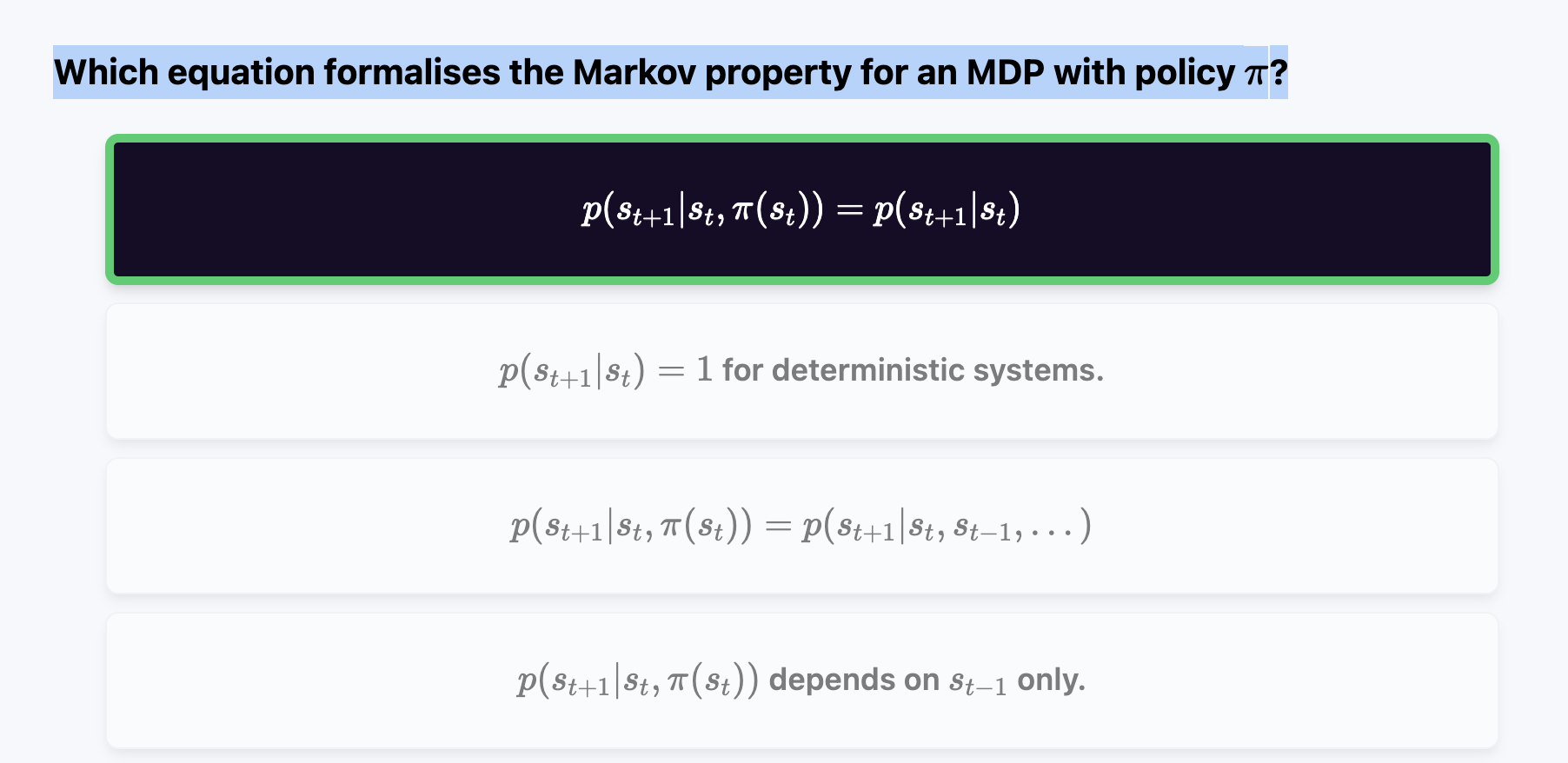
Which equation formalises the Markov property for an MDP with policy π?
- The next state 𝑆 𝑡 + 1 S t+1 depends only on the current state 𝑆 𝑡 S t and action 𝐴 𝑡 A t ,
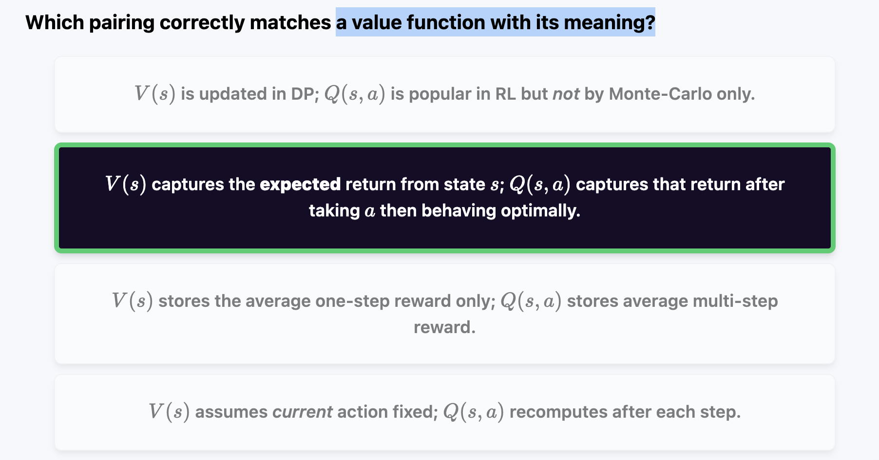
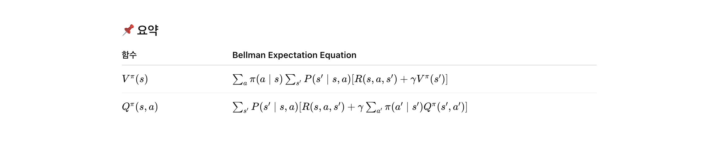
value function & meaning
-
State Value Function 𝑉 𝜋 ( 𝑠 ): 이 함수는 상태 𝑠 s에서 시작해서 정책 𝜋 π를 따랐을 때 얻을 것으로 기대되는 누적 보상의 기댓값
-
Action Value Function 𝑄 𝜋 ( 𝑠 , 𝑎 ) : 이 함수는 상태 𝑠 s에서 행동 𝑎 a를 취하고 이후 정책 𝜋 π를 따랐을 때 얻을 것으로 기대되는 보상의 기댓값
policy iteration steps + purpose
- policy evaluation : determin the state values for the given policy
- policy improvement : find a improved policy based on state values
Policy Iteration은 두 개의 반복 단계를 번갈아 수행하는 강화학습 알고리즘
✅ 1. Policy Evaluation 목적: 현재 정책 𝜋 하에서 각 상태의 가치 𝑉 𝜋 ( 𝑠 ) 를 계산하여, 정책이 얼마나 좋은지를 평가합니다.
✅ 2. Policy Improvement 목적: 각 상태에서 가장 좋은 행동을 선택하여 정책을 향상시키고, 더 나은 정책 𝜋 을 생성합니다.
Markov decision process MDP components in online scheduling
| 기호 | 설명 |
|---|---|
| S | 상태 집합 (State space): 에이전트가 있을 수 있는 모든 상태들 |
| A | 행동 집합 (Action space): 각 상태에서 취할 수 있는 행동들 |
| P | 상태 전이 확률 함수 (Transition probability): 특정 상태에서 어떤 행동을 했을 때 다음 상태로 갈 확률 |
| R | 보상 함수 (Reward function): 특정 상태에서 특정 행동을 했을 때 얻는 보상 |
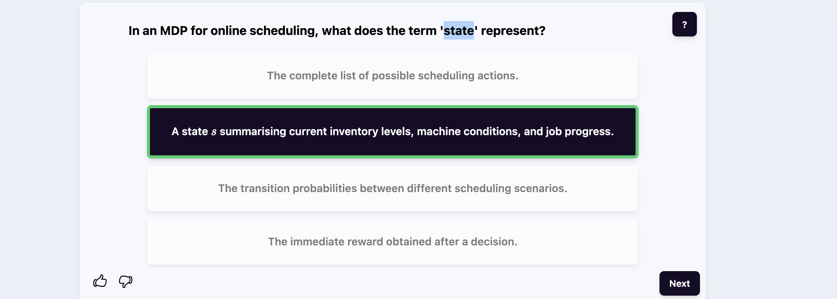
State Space (S):
Represents the current status of the system, such as machine availability, remaining processing times, job queues, or due dates.
Example: A state might encode which jobs are waiting and which machines are idle or busy.
Action Space (A):
The set of feasible scheduling decisions at each state, such as selecting which job to assign to which machine.
Example: Assigning job 3 to machine 2.
Transition Probability (P):
Describes the probability of moving from one state to another after an action is taken. In online scheduling, this may capture uncertainties like machine breakdowns or variable job processing times.
Example: With probability 0.9, a job completes on time; with 0.1, there's a delay due to unexpected setup.
Reward Function (R):
Assigns an immediate reward (or cost) to each state-action pair, guiding the system toward desirable behavior such as minimizing tardiness or makespan.
Example: A negative reward (i.e., penalty) for missing a due date or idling a machine.
!! While the discount factor is commonly used in reinforcement learning and discounted infinite-horizon MDPs, it is not always relevant in online scheduling problems that have a finite horizon
Differentiate between a decision/action and exogenous information in the MDP framework. -- 결정/행동과 외생 정보 (exogenous information)의 차이
- A decision/action is indeed something that the user can control,
- while exogenous information is outside the user's control, similar to the environment
In the MDP framework, a decision or action is a choice made by the agent in a given state—such as assigning a job to a machine—that directly influences the system's evolution. In contrast, exogenous information refers to stochastic events determined by the environment and outside the agent’s control, such as machine breakdowns, variable processing times, or new job arrivals. Importantly, exogenous information is typically revealed after an action is taken, and together they determine the transition to the next state. While decisions are deliberate and controllable, exogenous information introduces uncertainty, making planning under uncertainty essential in problems like online scheduling.
MDP의 불확실성은 전적으로 외생 정보에 의해 발생.
결정은 전략, 외생 정보는 리스크.
| 측면 | 결정 / 행동 | 외생 정보 |
|---|---|---|
| 통제 가능 여부 | ✅ 가능 | ❌ 불가능 |
| 결정 시점 | 에이전트가 먼저 선택 | 그 이후에 환경이 결정 |
| 역할 | 시스템 변화 유도 | 시스템의 불확실성 유발 |
| 영향 | 다음 상태 전이에 직접 영향 | 전이 확률을 결정함 |
Bellman Optimality Equation for MDP and role of each component
V(s)=maxa∈A{r(s,a)+γ∑s′p(s′∣s,a)V(s′)}.
- immediate reward
- discount factor
- transition probability

- 𝑉 ( 𝑠 ) V(s): 현재 상태 𝑠 s에서 얻을 수 있는 최대 기대 누적 보상 (가장 가치 있는 선택을 의미). max 𝑎 ∈ 𝐴 ( 𝑠 )
- max a∈A(s) : 가능한 모든 행동 𝑎 a 중에서 최적의 행동 선택 (예: 어떤 작업을 어떤 기계에 할당할지 결정).
- 𝑟 ( 𝑠 , 𝑎 ) r(s,a): 상태 𝑠 s에서 행동 𝑎 a를 취했을 때 얻는 즉시 보상 (예: 작업 완료로 인한 시간 절약 또는 벌점 회피).
- 𝛾 γ (Discount Factor): 미래 보상에 대한 현재 가치의 중요도를 결정. 0 ≤ 𝛾 ≤ 1 0≤γ≤1 (온라인 스케줄링에서 미래 작업의 영향까지 고려).
- ∑ 𝑠 ′ 𝑝 ( 𝑠 ′ ∣ 𝑠 , 𝑎 ) 𝑉 ( 𝑠 ′ ) ∑ s ′ p(s ′ ∣s,a)V(s ′ ): 행동 𝑎 a를 했을 때 다음 상태 𝑠 ′ s ′ 로 전이될 확률 가중치가 포함된 미래 가치의 합. (예: 기계 고장, 작업 지연과 같은 외생 정보를 반영한 불확실성 처리).
discound factor : How does the discount factor affect decisions in an infinite horizon MDP, and why is choosing a value less than one important?
- The discount factor down-weights future rewards, making sure that the infinite sum of returns converges to a finite value,
- which is essential for value iteration in an infinite-horizon MDP.
It scales future rewards ensuring convergence when 0<= r <1
state in MDP for online scheduling
advantage of online scheulding in manufacturing system
policy vs value iteration in MDP
Between value iteration and policy iteration for solving MDPs in online scheduling, which statement best captures a primary difference?
- policy iteration stops when the policy does not change, often converging faster in policy space
- Value iteration continuously updates value estimates to improve the policy indirectly,
- while policy iteration alternates between evaluating a fixed policy and explicitly improving it.
| Aspect | Value Iteration | Policy Iteration |
|---|---|---|
| Approach | Focuses on updating state values (V) | Focuses on improving the policy directly |
| Policy update | Derived indirectly from updated values | Explicitly updated after policy evaluation |
| Computation | Typically involves more iterations | Fewer iterations, but each step is more costly |
| Use case | Simple to implement, useful with large state spaces | Efficient when transitions and rewards are well-defined |
In an inventory MDP scenario, if the system state represents 'no inventory', what might be an optimal action as suggested by the lecture?
- Ordering enough to reach the target inventory level (e.g., maximum capacity or base-stock level).
- To minimize holding and shortage costs,
What role does the transition probability matrix play in an MDP used for online scheduling?
- it specifies the probability of moving from one state to another after an action
How can machine replacement decisions be modeled in an MDP framework in online scheduling?
- as actions that incur costs and change the state, with associated transition probabilities
Which two dynamic programming algorithms are highlighted in the lecture for solving MDPs in online scheduling?
- policy iteration, value iteration
Which statement best captures the exploration‑exploitation trade‑off in reinforcement learning (RL)?
- "Balancing the need to gather more information about the environment (exploration) with the goal of maximizing cumulative reward using known information (exploitation)."
Exploration: trying new or less-known actions to discover their potential long-term benefits.
Exploitation: choosing the currently best-known action to maximize immediate reward.
Summarize the key components of a policy function in the context of online scheduling with genetic programming and deep reinforcement learning.
The policy function uses state features to select actions based on learned rules (GP) or trained value/policy networks (DRL), aiming to optimize scheduling objectives in real-time.
Key Components:
1. State Representation (Input Features)
Describes the current status of the system.
Typical features include:
Remaining processing time of each job (RPT)
Time until due date (DD - CT)
Slack time ((DD - CT) - RPT)
Machine availability
Queue length at each machine
Operation count left for a job
- Action Space (Decisions)
Set of feasible dispatching rules or job selections.
Examples:
Select the job with shortest processing time (SPT)
Select the job with earliest due date (EDD)
Choose a job based on a learned priority function (via GP or DRL)
- Policy Function (Decision Rule)
In Genetic Programming: a symbolic expression tree combining features using operators (+, -, *, /, max, min)
E.g., 1.1 * PT - (DD - CT)
In Deep RL: a neural network that outputs action probabilities or values, trained through environment interaction.
- Reward Signal
Guides learning by quantifying decision quality.
Examples:
Negative makespan
Job lateness penalty
Weighted tardiness
Infix → Binary Tree
표현식 트리 변환 개요 (Infix → Binary Tree)
✅ 1. 중위 표기법 (Infix Notation)
우리가 수식을 보통 읽는 방식입니다.
예: 1.1 * PT - (DD - CT)
✅ 2. 접두 표기법 (Prefix Notation)
연산자를 먼저 쓰고, 피연산자를 그 뒤에 씁니다.
예: - * 1.1 PT - DD CT
→ 연산자 -가 먼저 나오고, 그 다음 항들이 차례로 따라옵니다.
✅ 3. 이진 트리로 변환
접두 표기(prefix)를 기반으로 다음과 같이 이진 트리를 만듭니다:
연산자는 내부 노드 (부모 노드)에 위치합니다.
피연산자(숫자, 변수)는 리프 노드 (말단 노드)에 위치합니다.