Forecast time series data!

1. Time series components

Time series 데이터에서 가장 중요한 것은 white noise를 찾아내는 것입니다. White noise는 시간에 따라 예측할 수 없는 무작위한 잡음을 나타내는 특별한 유형의 시계열 데이터입니다.

𝑋(t)가 다음 조건을 만족하면 white noise입니다.

1) $𝐸(𝑋(t)) = 0$
2) $𝐸(𝑋(t)^2) = \sigma^2$
3) $𝐸(𝑋(t)𝑋(h))=0 \space for \space t \neq h$.

즉, white noise는 평균이 0이며 분산이 상수이고 lag가 1이상일 때 autocorrelation이 0인 time series이며 weak stationarity 조건을 모두 만족합니다. 임의의 시계열 데이터에서 trend(추세)와 seasonality(계절성)을 제거하여 white noise를 얻어낼 수 있습니다. 아래는 그 예시를 나타내고 있습니다. 1년간 Apple의 Closing price를 trend와 seasonal로 분해하여 white noise를 만족하는 residual을 구해 plotting 한 소스코드와 그래프입니다.

from pandas import read_csv
from matplotlib import pyplot
from statsmodels.tsa.seasonal import seasonal_decompose

series = read_csv('./AAPL.csv', header = 0, index_col = 0, parse_dates = True)
series = series["Close"]
result = seasonal_decompose(series, model='additive', period = 7)

result.observed.rename_axis('Closing price')
result.seasonal.rename_axis('Seasonality')
result.resid.rename_axis('Risidual')
result.trend.rename_axis('Trend')
result.plot()

pyplot.show()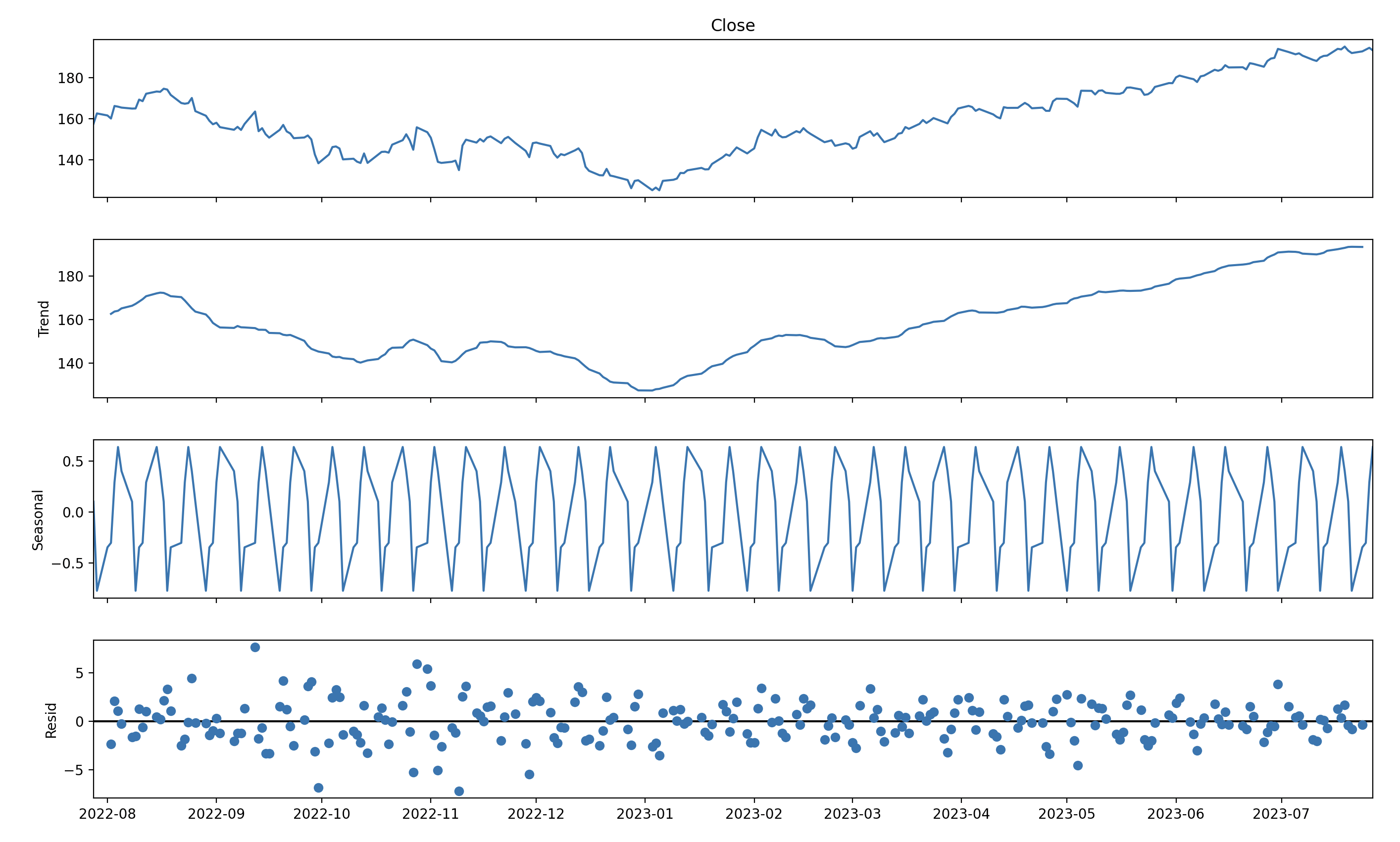

1) Trend(추세): 추세는 시간에 따라 데이터의 전반적인 방향성이나 경향성을 나타냅니다.
2) Seasonal(계절성): 계절성은 특정 시간 주기에 따라 주기적인 패턴을 나타냅니다. 주로 반복적인 변동성을 보이며, 일정한 시간 간격으로 주기적인 변동을 반복합니다.

2. Classical decomposition method

Classical decomposition method로는 additive와 multiplicative decomposition 둘로 나뉩니다. 관측한 시계열 데이터($y_t$)를 추세($T_t$), 계절성($S_t$), 잔차($R_t$)로 표현할 수 있습니다.

Decomposition

Additive and Multiplicative Decomposition는 각각 아래와 같이 표현할 수 있습니다.

$y_t = T_t + S_t + R_t$
$y_t = T_t S_t R_t$

여기서는 additive decomposition을 하는 방법만 간단하게 다루도록 하겠습니다. 아래의 step을 활용해서 additive decomposition을 진행할 수 있습니다.

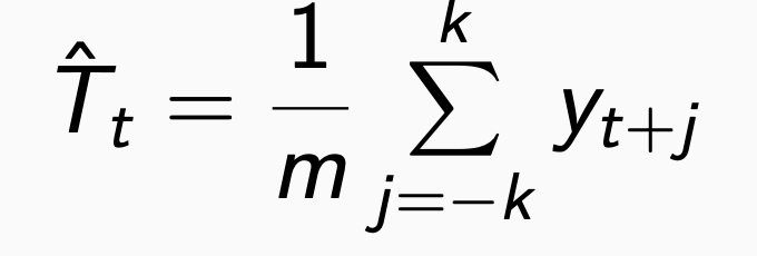
step 1: m이 짝수일때는 2 × m-MA, 홀수일때는 m-MA 방식을 활용해서 추세($T_t$)를 계산합니다.
step 2: 관측 시계열에서 추세를 제거합니다: $y_t - T_t$
step 3: 각 season에 대해서 평균을 취해 seasonality를 계산합니다.
step 4: 관측 시계열에서 추세와 계절성을 제거해 잔차를 구합니다.

m-MA 예시)

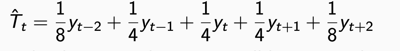
2 × m-MA 예시)

Forecasting

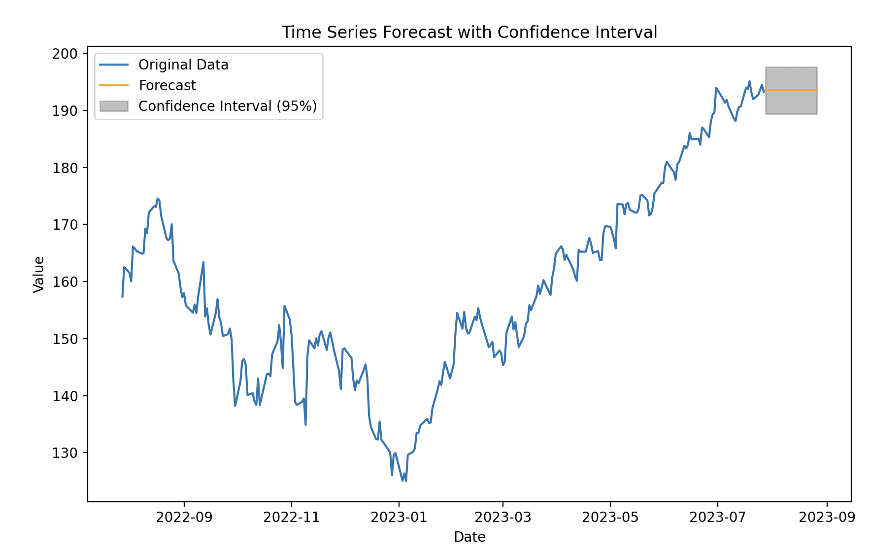
Classical decomposition method을 활용해서 forecasting 하는 방식은 드물게 활용되지만 그래도 confidence interval을 추정해서 데이터 예측에 관한insight를 얻을 수 있습니다. Error는 Normal distribution으로 가정했습니다. (더 정확히 예측하려면 t-distribution을 활용합니다.) z-test를 활용해 신뢰구간을 0.95로 설정하여 양측검정하면 예측값의 confidence interval을 구할 수 있습니다. 아래는 일련의 과정을 나타냅니다.

import pandas as pd
import matplotlib.pyplot as plt
from statsmodels.tsa.seasonal import seasonal_decompose
from pandas import read_csv

# 예시 데이터 생성 (날짜 및 시계열 값)
data = read_csv('./AAPL.csv', header = 0, index_col = 0, parse_dates = True)
data = data["Close"]

# 시계열 데이터 분해 (트렌드, 계절성, 잔차)
result = seasonal_decompose(data, model='additive', period=7)

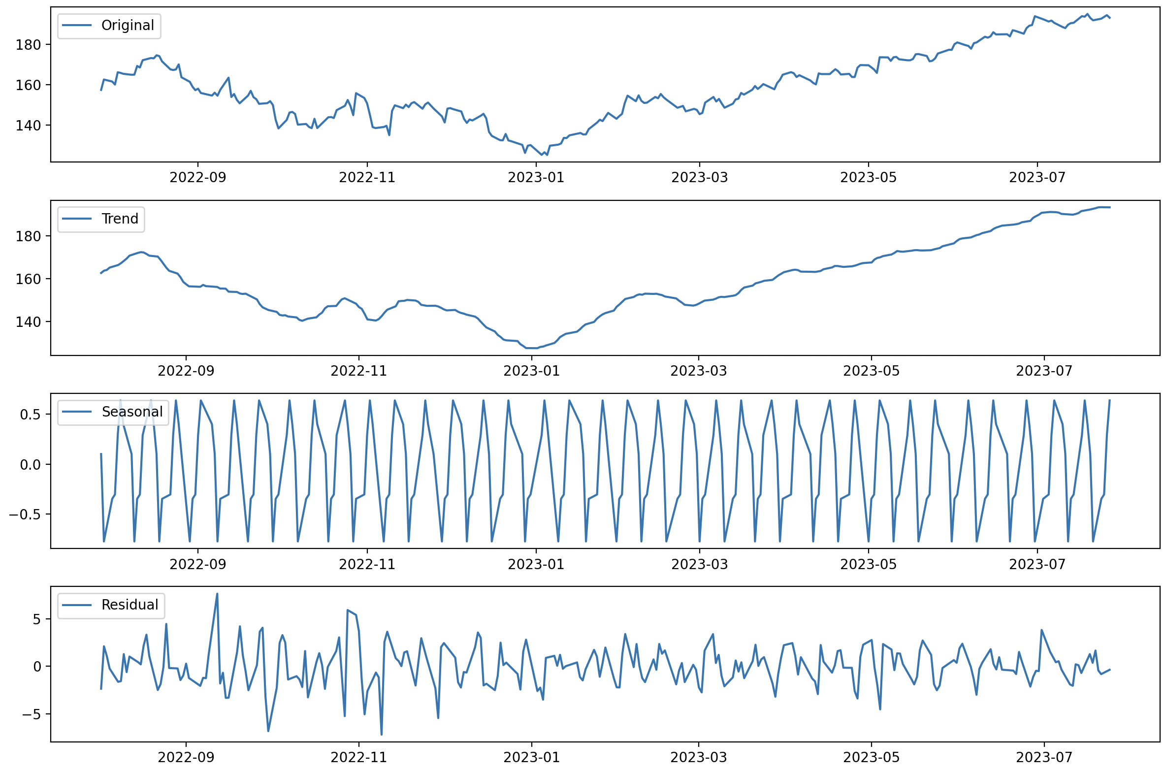
# 분해 결과 시각화
plt.figure(figsize=(12, 8))
plt.subplot(4, 1, 1)
plt.plot(data, label='Original')
plt.legend(loc='upper left')
plt.subplot(4, 1, 2)
plt.plot(result.trend, label='Trend')
plt.legend(loc='upper left')
plt.subplot(4, 1, 3)
plt.plot(result.seasonal, label='Seasonal')
plt.legend(loc='upper left')
plt.subplot(4, 1, 4)
plt.plot(result.resid, label='Residual')
plt.legend(loc='upper left')
plt.tight_layout()
plt.show()

# Forecast 함수 정의

# Forecast 함수 정의
def forecast(data, forecast_steps, confidence_interval=0.95):
    result = seasonal_decompose(data, model='additive', period=7)
    trend = result.trend.dropna()
    seasonal = result.seasonal.dropna()
    residuals = result.resid.dropna()

    # 잔차와 계절성 정보를 이용한 미래 값 예측
    forecasted_values = trend.iloc[-1] + seasonal[-forecast_steps:].mean() + residuals.mean()
    lower_bound = forecasted_values - residuals.std() * 1.96  # 95% 하위 신뢰구간
    upper_bound = forecasted_values + residuals.std() * 1.96  # 95% 상위 신뢰구간

    # Datetime Index를 만들어서 반환
    forecast_index = pd.date_range(start=data.index[-1] + pd.Timedelta(days=1), periods=forecast_steps, freq='D')
    forecast_series = pd.Series(forecasted_values, index=forecast_index)
    lower_bound_series = pd.Series(lower_bound, index=forecast_index)
    upper_bound_series = pd.Series(upper_bound, index=forecast_index)

    return forecast_series, lower_bound_series, upper_bound_series

# Forecast 함수 호출
forecast_steps = 30  # 30일 후 예측
forecast_series, lower_bound_series, upper_bound_series = forecast(data, forecast_steps)

# 결과 시각화
plt.figure(figsize=(10, 6))
plt.plot(data, label='Original Data')
plt.plot(forecast_series, label='Forecast', color='orange')
plt.fill_between(forecast_series.index, lower_bound_series, upper_bound_series, color='gray', alpha=0.5, label='Confidence Interval (95%)')
plt.legend(loc='upper left')
plt.xlabel('Date')
plt.ylabel('Value')
plt.title('Time Series Forecast with Confidence Interval')
plt.show()

마치며

원래는 X-11 decomposition, X-13ARIMA-SEATS decomposition, STL decomposition 등을 함께 다루고 ARIMA를 활용한 시계열 데이터 fitting을 계획했으나 시간관계상 다음 기회에 다루도록 하겠습니다.

당분간 https://brunch.co.kr/@gauss92tgrd/23 블로그를 살펴볼 예정입니다. 감사합니다.