모델을 구현하면서 논문 내용과 같이 살펴보겠습니다.
🔴 모델 구조
먼저 모델의 pretrained weight를 PyTorch에서 가져오겠습니다.
__all__ = [
    'VGG', 'vgg11', 'vgg11_bn', 'vgg13', 'vgg13_bn', 'vgg16', 'vgg16_bn',
    'vgg19_bn', 'vgg19',
]


model_urls = {
    'vgg11': 'https://download.pytorch.org/models/vgg11-bbd30ac9.pth',
    'vgg13': 'https://download.pytorch.org/models/vgg13-c768596a.pth',
    'vgg16': 'https://download.pytorch.org/models/vgg16-397923af.pth',
    'vgg19': 'https://download.pytorch.org/models/vgg19-dcbb9e9d.pth',
    'vgg11_bn': 'https://download.pytorch.org/models/vgg11_bn-6002323d.pth',
    'vgg13_bn': 'https://download.pytorch.org/models/vgg13_bn-abd245e5.pth',
    'vgg16_bn': 'https://download.pytorch.org/models/vgg16_bn-6c64b313.pth',
    'vgg19_bn': 'https://download.pytorch.org/models/vgg19_bn-c79401a0.pth',
}
왜 pretrained weight를 사용하나요?
👉 구현 검증, 성능 비교, 실용성을 위해
논문 수준의 성능을 처음부터 학습하려면 수일 ~ 수주가 걸릴 수 있습니다.
pretrained weight는 이미 대규모 데이터셋(ImageNet)에서 잘 학습된 값이므로 바로 fine-tuning이 가능합니다.
시간 & 자원 절약, 실험 반복을 위해 pretrained weight를 사용합니다.
VGG 논문에 기반한 모델 정의 클래스를 작성합니다.
class VGG(nn.Module):

    def __init__(self, features, num_classes=1000, init_weights=True):
    	super(VGG, self).__init__()
        self.features = features
        self.avgpool = nn.AdaptiveAvgPool2d((7, 7))
        self.classifier = nn.Sequential(
        	nn.Linear(512*7*7, 4096),
            nn.ReLU(),
            nn.Dropout(),
            nn.Linear(4096, 4096),
            nn.ReLU(),
            nn.Dropout(),
            nn.Linear(4096, num_classes))
        if init_weights:
        	self._initialize_weights()

    def forward(self, x):
    	x = self.features(x)
        x = self.avgpool(x)
        x = torch.flatten(x, 1)
        x = self.classifier(x)
        return x

    def _initialize_weights(self):
    	for m in self.modules():
        	if isinstance(m, nn.Conv2d):
            	nn.init.kaming_normal_(m.weight, mode='fan_out', nonlinearity='relu')
                if m.bias is not None:
                	nn.init.constant_(m.bias, 0)
            elif isinstance(m, nn.BatchNorm2d):
            	nn.init.constant_(m.weight, 1)
                nn.init.constant_(m.bias, 0)
            elif isinstance(m, nn.Linear):
            	nn.init.normal_(m.weight, 0, 0.01)
                nn.init.constant_(m.bias, 0)
☑️ 주목해야할 점
1️⃣ 각각의 모듈에 대해 초기화 방식 다르게 적용
참고: 논문 내에서 kaiming 초기화, BatchNorm 사용은 언급되지 않았습니다.
| Layer Type | Weight Initialization | Bias Initialization | Rationale |
|---|---|---|---|
nn.Conv2d | kaiming_normal_ (mode='fan_out', relu) | 0 | ReLU는 음수를 죽이므로 분산 조절 필요 (He 초기화) |
nn.BatchNorm2d | Constant 1 | 0 | 초기에는 정규화된 출력을 그대로 전달 (y = x) |
nn.Linear | Normal(mean=0, std=0.01) | 0 | 논문에서 FC layer는 이렇게 초기화한다고 명시 |
"The weights are initialized with a normal distribution (mean 0, standard deviation 0.01). Biases are initialized with 0."
2️⃣ 처음 두 개의 FC layer에 Dropout 정규화 (0.5)
"Dropout regularization was used for the first two fully connected layers with dropout ratio set to 0.5."
VGG 구조의 깊이에 따라 다양한 구성에 대응할 수 있도록 계층을 동적으로 생성하는 함수를 구현해보겠습니다.
def make_layers(cfg, batch_norm=False):
	layers = []
    in_channels = 3
    for v in cfg:
    	if v == 'M':
        	layers += [nn.MaxPool2d(kernel_size=2, stride=2)]
        else:
        	conv2d = nn.Conv2d(in_channels, v, kernel_size=3, padding=1)
         	if batch_norm:
            	layers += [conv2d, nn.BatchNorm2d(v), nn.ReLU(inplace=True)]
            else:
            	layers += [conv2d, nn.ReLU(inplace=True)]
            in_channels = v
    return nn.Sequential(*layer)
☑️ 주목해야할 점
1️⃣ 입력 이미지는 224x224 크기의 RGB 이미지
"The only pre-processing we do is subtracting the mean RGB value, computed on the training set, from each pixel. The input to our ConvNets is a fixed-size 224 × 224 RGB image."
2️⃣ 활성화 함수는 ReLU
"All hidden layers are equipped with the rectification (ReLU [7]) non-linearity.”
3️⃣ stride와 padding을 고정해 resolution 유지
"The convolution stride is fixed to 1 pixel; the spatial padding of conv. layer input is such that the spatial resolution is preserved after convolution, i.e. the padding is 1 pixel for 3 × 3 conv. layers."
4️⃣ 모든 convolution layer는 3x3 kernel
“We use very small convolution filters: 3 × 3 with stride 1 and pad 1.”
왜 3 x 3 커널만 사용하나요?
VGG 논문에서 (3 x 3) 필터 사용의 효과를 평가한 실험 결과를 제시했습니다.
실험 3: (3 x 3) 필터의 장점
논문에서는 큰 필터(예: 5x5, 7x7)를 사용하는 대신, 여러 개의 3x3 필터를 연속적으로 사용하는 것이 파라미터 수를 줄이면서도 성능을 향상시킬 수 있음을 강조합니다.
“Stacking three 3×3 conv. layers (without spatial pooling in between) is in terms of effective receptive field equivalent to a single 7×7 conv. layer. More importantly, it increases the number of nonlinearities, making the decision function more discriminative.”
“For instance, a stack of two 3×3 conv. layers has an effective receptive field of 5×5 three such layers have a 7×7 effective receptive field. More importantly, the use of multiple small filters increases the number of nonlinearities, which makes the decision function more discriminative.”
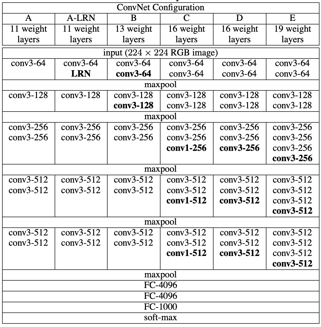
VGG는 깊이에 따라 여러 버전(A~E)의 모델 구성이 존재합니다.
각 구성은 Conv 레이어의 개수와 배열이 다르기 때문에 이를 리스트 형태로 정의하겠습니다.
이 리스트는 이후 make_layers() 함수에서 실제 레이어를 생성할 때 참조됩니다.
cfgs = {
    'A': [64, 'M', 128, 'M', 256, 256, 'M', 512, 512, 'M', 512, 512, 'M'],
    'B': [64, 64, 'M', 128, 128, 'M', 256, 256, 'M', 512, 512, 'M', 512, 512, 'M'],
    'D': [64, 64, 'M', 128, 128, 'M', 256, 256, 256, 'M', 512, 512, 512, 'M', 512, 512, 512, 'M'],
    'E': [64, 64, 'M', 128, 128, 'M', 256, 256, 256, 256, 'M', 512, 512, 512, 512, 'M', 512, 512, 512, 512, 'M'],
}
☑️ 주목해야할 점
1️⃣ LRN 실험
LRN은 정확도 향상에 기여하지 않으며 오히려 메모리 사용량과 계산 시간을 증가시키는 것으로 나타났습니다.
“We note that none of our networks (except for one) contain Local Response Normalisation (LRN) normalisation (Krizhevsky et al., 2012): as will be shown in Sect. 4, such normalisation does not improve the performance on the ILSVRC dataset, but leads to increased memory consumption and computation time.”
2️⃣ Conv 1 x 1 실험
1 x 1 conv를 포함한 구성은 동일한 깊이의 3 x 3 conv만을 사용한 구성보다 성능이 낮았습니다. 1 x 1 conv이 비선형성은 증가시키지만 공간적 정보를 포착하는 데에는 한계가 있음을 의미합니다.
“Although 1×1 convolutions can be used to change the dimensionality of the filter space, in VGGNet they were added to increase the non-linearity of the decision function without modifying the receptive field.”
“The configurations with 1×1 convolutional layers perform worse than the equivalent configurations with 3×3 kernels. They conclude that even though 1×1 convolutions help (as C performs better than B), it is important to capture the spatial context by using convolutional filters (D performs better than C).”
각 모델들의 구성 및 weight 불러오는 과정을 공통으로 처리하는 함수를 정의하겠습니다.
def _vgg(arch, cfg, batch_norm, pretrained, progress, **kwargs):
    if pretrained:
        kwargs['init_weights'] = False
    model = VGG(make_layers(cfgs[cfg], batch_norm=batch_norm), **kwargs)
    if pretrained:
        state_dict = load_state_dict_from_url(model_urls[arch],
                                              progress=progress)
        model.load_state_dict(state_dict)
    return model
VGG11, 13, 16, 19를 정의하겠습니다.
def vgg11(pretrained=False, progress=True, **kwargs):
	return _vgg('vgg11', 'A', False, pretrained, progress, **kwargs)

def vgg11_bn(pretrained=False, progress=True, **kwargs):
	return _vgg('vgg11_bn', 'A', True, pretrained, progress, **kwargs)

def vgg13(pretrained=False, progress=True, **kwargs):
	return _vgg('vgg13', 'B', False, pretrained, progress, **kwargs)

def vgg16(pretrained=False, progress=True, **kwargs):
	return _vgg('vgg16', 'D', False, pretrained, progress, **kwargs)

def vgg19(pretrained=False, progress=True, **kwargs):
	return _vgg('vgg19', 'E', False, pretrained, progress, **kwargs)
이렇게 해서 VGG 모델 구현은 완료했습니다.
VGG 핵심 특징
• 모든 Conv 필터 3x3 고정
• 네트워크 깊이만 점진적으로 증가 (최대 19층)
• FC -> Conv 변환으로 Dense Evaluation
• Scale Jittering & Multi-crop 등 다양한 평가 전략 도입
• 단순한 구조로도 GoogLeNet에 근접한 성능 달성
이외 논문에 기재된 나머지 특이사항을 짚어보겠습니다.
🔴 Training Data Preprocessing
VGG 논문에서는 모든 입력 이미지를 224×224 크기의 RGB 이미지로 고정하고 각 픽셀에서 훈련 세트의 평균 RGB 값을 빼는 방식으로 정규화를 수행했습니다.
"The input to our ConvNets is a fixed-size 224 × 224 RGB image."
"The only pre-processing we do is subtracting the mean RGB value..."
preprocess = transforms.Compose([
    transforms.Resize(256),               # S = 256 (isotropic resize, 짧은 변 기준)
    transforms.CenterCrop(224),           # 항상 224x224로 crop
    transforms.ToTensor(),                # [0,255] → [0,1]
    transforms.Normalize(                 # VGG 논문 기준 평균 RGB 값
        mean=[0.485, 0.456, 0.406],       # ImageNet 훈련셋 평균
        std=[0.229, 0.224, 0.225]         # ImageNet 훈련셋 표준편차
    )
])
논문에서는 "mean RGB subtraction"만 언급했지만 PyTorch pretrained 모델들과 호환하려면 Normalize(mean, std)를 사용하는 것이 일반적입니다.
(Resize에 대한 실험은 아래에서 다룹니다.)
🔴 Training Settings
VGG는 논문에서 다음과 같은 학습 설정을 사용했습니다.
| 항목 | 값 |
|---|---|
| Optimizer | SGD with momentum |
| Momentum | 0.9 |
| Weight Decay | 5×10⁻⁴ |
| Batch size | 256 |
| Learning rate | 초기 10⁻², 성능 개선 없을 시 3번 감쇠 |
| Dropout | FC 레이어 앞에 0.5 |
| Iterations | 370,000 (74 epochs) |
| 초기화 전략 | 얕은 네트워크 → 깊은 네트워크 초기화 |
왜 Deep Network인데도 수렴이 빨랐는가?
암시적 정규화(implicit regularisation) + 얕은 네트워크 가중치로 초기화
"Despite the large number of parameters and depth, our networks do not suffer from overfitting, possibly due to implicit regularisation from small convolution filters."
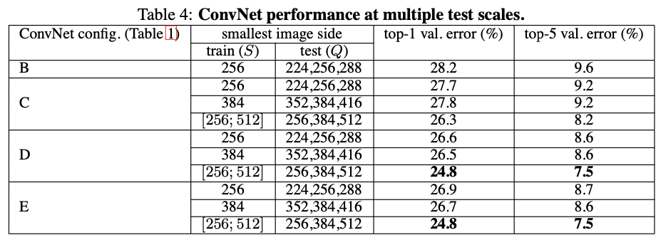
🔴 Training Image Scale 실험 (S 실험)
VGG에서는 입력 이미지의 크기(S)를 달리 해 학습한 후 성능 차이를 비교했습니다.
| 전략 | 설명 |
|---|---|
| Single-scale (S=256 or 384) | 고정된 이미지 크기로 학습 |
| Multi-scale ([256, 512]) | 각 에폭마다 S를 랜덤하게 샘플링 |
결과적으로 multi-scale 학습이 다양한 물체 크기에 robust한 feature를 만들어 성능이 더 높았습니다.
1️⃣ 고정 범위에서 학습한 경우(Single-Scale Training)
“For single-scale training, we fix S and then evaluate the model at scales S−32, S, and S+32.”
2️⃣ 다중 스케일로 학습한 경우(Multi-Scale Training)
“For multi-scale training, we evaluate the model at the minimum, median, and maximum scales used during training.”

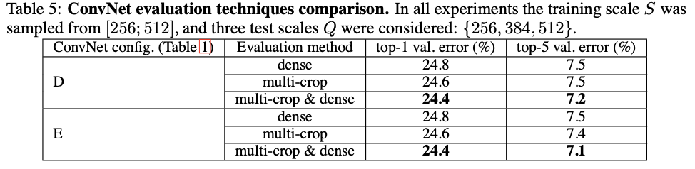
🔴 Test-time Settings
VGG 논문에서는 다음과 같은 다양한 테스트 전략을 실험했습니다.
1️⃣ Dense Evaluation
FC layer를 Conv layer로 변환하여 입력 이미지 전체에 ConvNet을 sliding window 방식으로 적용하는 전략입니다.
“At test time, the fully connected layers are converted to convolutional layers, allowing the network to be applied to images of arbitrary size in a fully convolutional fashion. The class scores are then obtained by spatially averaging the output maps.”
2️⃣ Multi-scale Evaluation
하나의 이미지에 대해 여러 해상도(Q ∈ {256, 384, 512})로 resize하여 각각 Dense Evaluation을 수행한 뒤 각 스케일에서의 예측 결과를 평균(ensemble)합니다.
“We also evaluate the networks at multiple scales by resizing the input images to different scales and averaging the predictions.”
3️⃣ Multi-crop Evaluation
각 이미지에서 25개의 crop을 추출하고, 수평 뒤집기(flip)를 적용하여 총 50개의 crop 평가했습니다. 이 과정을 세 가지 스케일에서 반복하여 총 150개의 crop을 평가합니다.
“In addition to the dense evaluation, we also evaluate multi-crop settings by sampling multiple crops (5 × 5 grid with 2 × flip = 50 crops) at each of 3 scales.” (Q ∈ {256, 384, 512})
4️⃣ Dense + Multi-crop Ensemble
위 두 방법(Dense Evaluation + Multi-crop Evaluation)의 결과를 결합하여 앙상블한 방식입니다.
이 전략은 VGG 최종 모델의 성능을 극대화했으며 Top-5 오류율 6.8%를 기록했습니다.
“Combining the dense and multi-crop evaluations further improves the performance, achieving a top-5 error rate of 6.8%.”
🔴 VGG vs GoogLeNet
| 항목 | VGG | GoogLeNet |
|---|---|---|
| Top-5 오류율 | 6.8% | 6.7% |
| 구조 | 순차적, 단순 | Inception 모듈, 병렬적 |
| 필터 종류 | 주로 3×3 | 1×1, 3×3, 5×5 혼합 |
| 특징 | 깊이 위주 | 차원 축소 + 멀티스케일 특징 |