librosa - 음정 유사도 비교하기

띠용·2024년 8월 19일

졸업 프로젝트 : AI 보컬 커버 & 트레이닝

목록 보기

2/3

1번 음악이 기준이 될 저스디스의 너의 모든 순간 커버 음원이다.
배경음이 비교적 없고 깔끔한 것 같아서 기준으로 선정함.
https://www.youtube.com/shorts/FOLOE5zd8y8

2번 음악은 잘 부른 예시. 유튜브에서 일반인 커버 영상을 따왔다.
https://www.youtube.com/shorts/5BPzkbZtHf8

3번은 집에서 놀던 동생한테 따라서 불러보라고 한 녹음 파일이다.
미안하지만 아쉬운 예시로 선정했다.

1번과 2번은 무료 웹사이트를 통해 mr을 제거했다.

# 오디오 파일 로드
y1, sr1 = librosa.load('/content/drive/MyDrive/Colab Notebooks/audio_processing/저스디스mr제거.mp3')
y2, sr2 = librosa.load('/content/drive/MyDrive/Colab Notebooks/audio_processing/일반인_무반주.mp3')
y3, sr3 = librosa.load('/content/drive/MyDrive/Colab Notebooks/audio_processing/시은이.mp3')

# 기본 주파수 추정
f0, voiced_flag, voiced_probs = librosa.pyin(y1,sr=sr1, fmin = librosa.note_to_hz('C2'), fmax=librosa.note_to_hz('C7'))
f0_2, voiced_flag_2, voiced_probs_2 = librosa.pyin(y2, sr = sr2, fmin = librosa.note_to_hz('C2'), fmax=librosa.note_to_hz('C7'))
f0_3, voiced_flag_2, voiced_probs_3 = librosa.pyin(y3, sr = sr3, fmin = librosa.note_to_hz('C2'), fmax = librosa.note_to_hz('C7'))

# NaN 값을 선형 보간법으로 채우기
f0_interpolated = pd.Series(f0).interpolate().to_numpy()
f0_2_interpolated = pd.Series(f0_2).interpolate().to_numpy()
f0_3_interpolated = pd.Series(f0_3).interpolate().to_numpy()

오디오 파일 준비

librosa.load - 오디오 원음 파일(시간대 별 진폭 데이터)과 샘플링 레이트를 로드한다.

librosa.pyin - 시간대별 주파수 데이터를 획득, f0 = 특정 시간 구간에서 오디오 신호의 주된 진동수를 나타냄

만약 해당 구간에서 주파수를 추정할 수 없는 경우 'NaN'값이 저장된다.

NaN값이 존재하면 비교 연산에 방해가 되기 때문에 빈 값이 없게 적당히 채워줄 것이다.

NaN 값을 선형보간법으로 어림잡아 채운다. (interpolated), 빠른 배열간 연산을 위해 numpy화 한다.
하지만 선형보간법을 적용할 수 없어 남아있는 NaN값들은 존재한다.

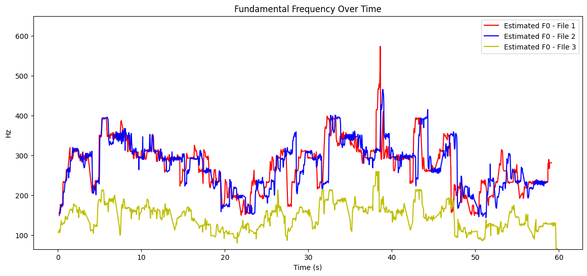
그래프 그리기

# 시간 축 계산
times = librosa.times_like(f0, sr=sr1)
times_2 = librosa.times_like(f0_2, sr=sr2)
times_3 = librosa.times_like(f0_3, sr=sr3)

# 그래프로 주파수 시각화
plt.figure(figsize=(14, 6))
plt.plot(times, f0_interpolated, label='Estimated F0 - File 1', color='r')
plt.plot(times_2, f0_2_interpolated, label='Estimated F0 - File 2', color='b')
plt.plot(times_3, f0_3_interpolated, label='Estimated F0 - FIle 3', color = 'y')

plt.xlabel('Time (s)')
plt.ylabel('Hz')
plt.title('Fundamental Frequency Over Time')
plt.ylim([librosa.note_to_hz('C2'), 650])
plt.legend()
plt.show()

times_like로 음원의 주파수 별 시간 값을 반환

plot으로 x축에 times, y축에 선형보간처리 한 주파수 데이터를 넣고 그린다.

유사도 비교

import numpy as np
import pandas as pd
import librosa

def compare_music(music_1, music_2):
  # 두 주파수 데이터의 최소 길이 맞추기
  min_length = min(len(music_1), len(music_2))
  music_1 = music_1[:min_length]
  music_2 = music_2[:min_length]

  # NaN 값이 있는 인덱스 제거
  valid_idx = ~np.isnan(music_1) & ~np.isnan(music_2)
  music_1_valid = music_1[valid_idx]
  music_2_valid = music_2[valid_idx]

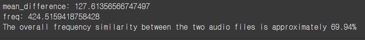
  # 두 주파수 값의 차이 계산
  f0_difference = np.abs(music_1_valid - music_2_valid)

  # 평균 절대 차이 계산
  mean_difference = np.mean(f0_difference)
  print("mean_difference:", mean_difference)
  
  # 최대 주파수 범위
  freq_scope =  max(music_1_valid) - min(music_1_valid)
  print("freq:", freq_scope)
  
  # 유사도 계산 (1-(평균 차이 / 주파수 범위))
  similarity = (1 - (mean_difference / freq_scope)) * 100
  print(f'The overall frequency similarity between the two audio files is approximately {similarity:.2f}%')

compare_music(music_1=f0_interpolated, music_2=f0_2_interpolated)