1. 구간분할
-
데이터 분석 알고리즘에 따라서는 연속 데이터를 그대로 사용하기 보다는 일정한 구간(bin)으로 나눠서 분석하는 것이 효율적인 경우가 있다.
-
가격이나 비용, 효율 등 연속적인 값을 일정한 수준이나 정도를 나타내는 이산적인 값으로 나타내어 구간별 차이를 드러내는 것이다
-
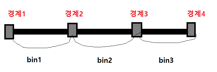
이처럼 연속 변수를 일정한 구간으로 나누고, 각 구간을 범주형 이산변수로 변환하는 과정을 구간 분할(binning) 이라고 한다.
-
판다스의 cut() 함수 를 이용하여 연속데이터를 여러구간으로 나누고 범주형 데이터로 변환할 수 있다.
import pandas as pd
import numpy as np

df = pd.read_csv(r'C:\Users\kjt63\OneDrive\바탕 화면\python\data_analysis\sample\part5\auto-mpg.csv',header=None)

df.columns= [ 'mpg','cylinders','displacement','horsepower','weight','acceleration','model year','origin','name']


# horsepower 열의 누락데이터('?')를 삭제하고 실수형을 변환

df['horsepower'].replace('?',np.nan,inplace=True)
df.dropna(subset=['horsepower'],axis=0,how='any',inplace=True)
df['horsepower']= df['horsepower'].astype('float')


# np.histogram 함수로 3개의 bin으로 구분할 경계값의 리스트 구하기

count, bin_dividers = np.histogram(df['horsepower'],bins=3)

print(count)

print(bin_dividers)


# count = [257 103  32]

# bin_dividers =[ 46.         107.33333333 168.66666667 230.        ]

# 4개의 경곗값 3개의 구간이 만들어짐
#                      ( 46 ~ 107.3,
#                       107.3~168.6,
#                       168.6~230)

bin_names = ['저출력','보통출력','고출력']

df['hp_bin'] = pd.cut(df['horsepower'], # 데이터 배열
                        bins=bin_dividers, #  경계값 리스트
                        labels = bin_names, # bin이름
                        include_lowest = True) # 첫 경곗값 포함


print(df[['horsepower','hp_bin']].head(15))
   [257 103  32]
   [ 46.         107.33333333 168.66666667 230.        ]
   horsepower hp_bin
    0        130.0   보통출력
    1        165.0   보통출력
    2        150.0   보통출력
    3        150.0   보통출력
    4        140.0   보통출력
    5        198.0    고출력
    6        220.0    고출력
    7        215.0    고출력
    8        225.0    고출력
    9        190.0    고출력
    10       170.0    고출력
    11       160.0   보통출력
    12       150.0   보통출력
    13       225.0    고출력
    14        95.0    저출력
2. 더미 변수
- 앞에서 'horsepower' 열의 숫자형 연속 데이터를 'hp_bin' 열의 범주형 데이터로 변환하였다. 하지만 이처럼 범주형 데이터를 회귀분석 등
머신러닝 알고리즘에 바로 사용할 수 없는 경우가 있는데, 컴퓨터가 인식 가능한 입력값으로 변환해야 한다. - 이럴 때 숫자 0 또는 1로 표현되는 더미변수(dummy variable)를 사용한다.
-
여기서 0과 1은 수의 크고 작음을 나타내지 않고, 어떤 특성의 존재여부를 표시한다.
-
get_dummies() 함수를 사용하면 범주형 변수의 모든 고유값을 각각 새로운 더미 변수로 변환한다.
import pandas as pd
import numpy as np

df = pd.read_csv(r'C:\Users\kjt63\OneDrive\바탕 화면\python\data_analysis\sample\part5\auto-mpg.csv',header=None)

# 열 이름 지정
df.columns= [ 'mpg','cylinders','displacement','horsepower','weight','acceleration','model year','origin','name']

# horsepower 열의 누락데이터('?')를 삭제하고 실수형을 변환
df['horsepower'].replace('?',np.nan,inplace=True)
df.dropna(subset=['horsepower'],axis=0,how='any',inplace=True)
df['horsepower']= df['horsepower'].astype('float')


count, bin_dividers = np.histogram(df['horsepower'],bins=3)

bins_name = [ '저출력','보통출력','고출력']

df['hp_bin']=pd.cut(df['horsepower'],bins=bin_dividers, labels=bins_name,include_lowest=True)


# get_dummies() 함수를 사용하여 열의 고유값 3개가 각각 새로운 더미 변수열의 이름이 된다.
horsepower_dummies = pd.get_dummies(df['hp_bin'])
print(horsepower_dummies.head(15))
    저출력  보통출력  고출력
0     0     1    0
1     0     1    0
2     0     1    0
3     0     1    0
4     0     1    0
5     0     0    1
6     0     0    1
7     0     0    1
8     0     0    1
9     0     0    1
10    0     0    1
11    0     1    0
12    0     1    0
13    0     0    1
14    1     0    0
※ sklearn 라이브러리를 이용해서 원핫인코딩을 편하게 처리할 수 있다.
# 데이터프레임 df의 'hp_bin'열에 들어있는
범주형 데이터를 0,1을 원소로 갖는 원핫벡터로 변환한다.
결과는 희소행렬(Sparse Matrix)로 정리된다

# 희소행렬은 (행,열) 좌표와 값 형태로 정리된다.


from sklearn import preprocessing

# 전처리를 위한 encoder 객체 만들기
label_encoder = preprocessing.LabelEncoder() # label_encoder 객체생성
onehot_ enocoder = preprocessing.OneHotEncoder() # onehot_encoder 생성

# label encoder 로 문자열 범주를 숫자형 범주로 변경
onehot_labeled = label_encoder.fit_transform(df['hp_bin'].head(15))
print(onehot_labeled)
print(type(onehot_labled))

# 2차원 행렬로 변경
onehot_reshaped = onehot_labeled.reshpae(len(onehot_labeled),1)
print(onehot_reshaped)
print(type(onehot_reshaped))

# 희소행렬로 변경
one_fitted = onehot_encoder.fit_transform(onehot_reshaped)
print(onehot_fitted)
print(type(onehot_fitted))