Day1

🟢 온라인 노트북

코랩, runpod

• gpu 잘 사용하는 방법

AWS SageMaker

• 아마존에서 제공하는 노트북

🟢머신러닝 개요

🔵고양이와 강아지를 구분해본다…

feature(특성), columns, x값, 설명변수

• 색, 몸무게, 키, 수염 개수, 눈 크기….
• 특성의 개수 = 차원의 개수
• 여러 건의 데이터 ⇒ rows, 관측 데이터
• 모두 스칼라 값이라는 가정 하에 벡터가 됨 ⇒ 차원 축소 가능

종류, y값 , target, label, 종속변수

강아지, 고양이.

🔵10차원 → 2차원 축소 (PCA)

• 선형대수 기반. eigen vector와 eigen value의 분산이 큰 방향으로 축소
• 2차원에 있다는 가정 하에 직선으로 강아지와 고양이를 구분
• 그 직선을 방정식으로 y= ax+b
• a → weight(가중치), b → bias(편향)

🔵강아지와 고양이를 구분하는 과정(분류)

• train(학습) → 시행착오
• 이것은 정답이 있으므로 지도학습(labeling 필요, 데이터 바우처 사업)
• 없으면 비지도학습
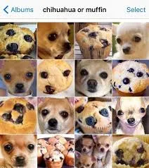
• 과적합 주의.(overfitting) ⇒ 훈련만 잘 되고, 예측을 못함.

🔵gpt

• AI는 결국 수식이다. gpt는 수식이 아주 복잡할 뿐이다.
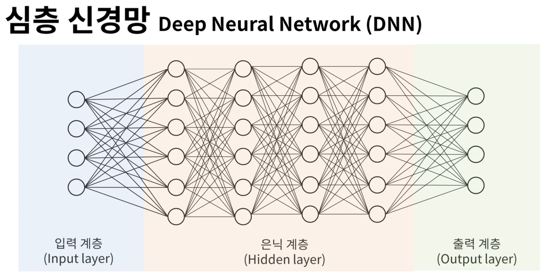
• DNN 사용 → 간선 하나하나가 y=ax+b

🔵NVIDIA 프로세서

cuda 프로세서로 돌아감.

🔵회귀

• 숫자를 맞추면 회귀
• 둘 중 하나를 맞추면 분류.

공분산 ⇒ 단위 존재

상관계수 ⇒ 단위 X, 방향만 남음.

• 선형회귀(통계학) = 직선 방정식? = 선형결합은 선형이다.

🔵비선형회귀

• 딥러닝은 대표적인 비선형 모델
• 선형과 선형을 더하면 선형이어야하는데? → 비선형처리하는 도구가 필요
  - 활성화 함수
  

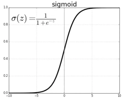
• e의 지수 -z에는 ax+b가 들어가 있음
• 시그모이드 함수는 로지스틱 회귀 문제에도 사용됨. ⇒ 0과 1을 출력할 수 있음.
• 활성화 함수는 각 노드별로 각각 붙어있어 출력 시 처리된다.

🟢 머신러닝의 목적

🔵결국 하려는 것은?

• w,b ⇒ 시행착오(학습) , 데이터를 표현할 w,b 찾기
• 회귀식 - 라벨값 = error(오차)

🔵오차를 다룬다.

• 회귀식 때는 오차의 합이 줄어들게 접근해야 함.
• error sum의 평균 → Mean 편차(오차)의 제곱의 루트 ⇒ Mean Square Error(MSE)
  • 작게 하는 방향으로 계속 갈굼.
  • 너무 갈구면 과적합 될 수 있으므로 trade-off의 관계를 보임.

🔵학습을 한 번만 할 수는 없다

• dataset 한 번 다 소비 ⇒ 1 epoch → 하이퍼파라미터(사람이 고름)

🔵편향(bias) 종류

• 확증 편향

  • 자신이 믿고 있는 그대로, 받아들이고 싶어하는 편향

• 기준점 편향

  • 분석가가 처음 접해보는 정보에 지나치게 매몰되는 편향
  • 연인 선물

• 선택 지원 편향

  • 본인이 의사결정을 내리는 순간 그 선택의 긍정적인 부분에 대해 더 많이 생각함.
  • 결국 그 결정의 반대에 대해 무시해버리는 편향

• 생존자 편향

  • 살아있는 사람에 대해 정보를 분석하여 본질을 못잡은 편향

• 서적 추천 : 가볍게 시작하는 통계학습. 근데 번역이 나쁨

https://www.statlearning.com/

갑자기 pdf 추천. 다운로드 받긴 했어요

🔵평가지표

함수에 hat? → 예측값.

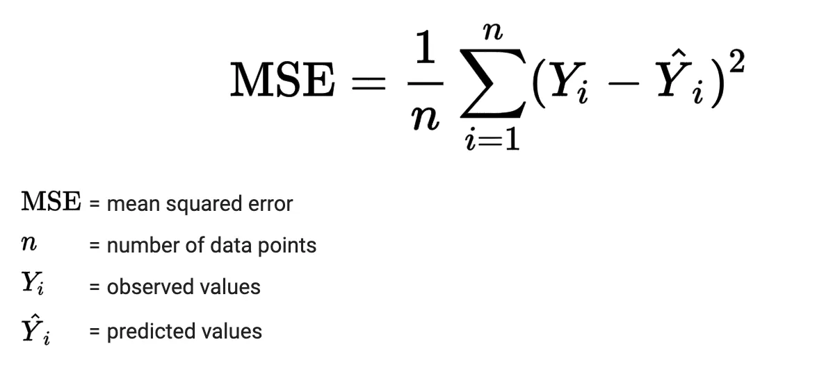
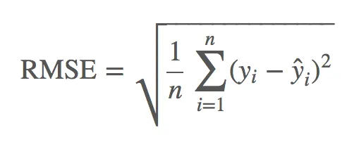
• MSE 값이 크다는 것은 잘못된 학습이라는 뜻
• RMSE → MSE에 루트 덮는 것.

분류 테스크

• 정보 엔트로피 공식
• 지니계수

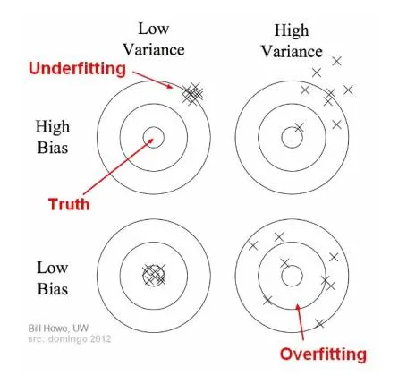
분산 편향 trade off

사이킷런을 시작한다…

https://scikit-learn.org/stable/

• 비지도학습 : 클러스터링.
• 차원 축소도 대표적인 비지도학습(x값을 줄인다.)

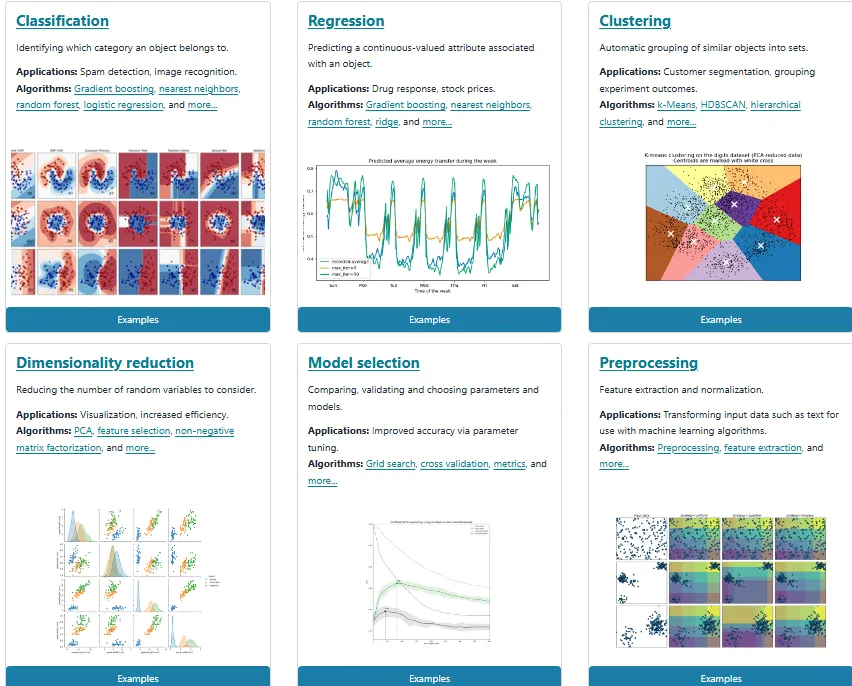
• preprocessing ⇒ 원핫인코딩, 라벨인코딩을 돕는 라이브러리 존재.

🟢Deep Learning

딥러닝 → tensorflow(google) → tensorflow 2.20.0

tensorflow는 버전별로 문제가 많음. 이걸 해결하기 위해 keras 도입.

cuda 생태계 ⇒ nvidia

TPU → 구글이 딥러닝 할 때. gemini 3 .

• arm 아키텍쳐
• apple silicon → m4
• Metal.

META- pytorch → LLM의 발전으로 점유율 확장

• class, generator 이해.

🔵간단한 딥러닝 모델 소개

• DNN
  • 분류, 회귀 사용
• CNN
  • DNN+(convolution) ⇒ CNN
  • 이미지 특화 모델
  • 이미지의 특징 추출.
  • 성능이 높은 편.

• RNN
  • 시계열 데이터에 특화되어있음.
  • 번역, 음성인식 → transformer로의 확장

🔵검색엔진(구글, 야후 등등)

• 크롤러를 만들어.
• robots.txt → 약속.

🔵GPT

• Generative Pre-trained Transformer

🟢사이킷런을 시작한다.

• 선형대수적 태스크는 np로 해결한다.

np.arange(20).reshape(2,10)
np.arange(20).reshape(-1,10)

array([[ 0, 1, 2, 3, 4, 5, 6, 7, 8, 9],
[10, 11, 12, 13, 14, 15, 16, 17, 18, 19]])

• 앞 쪽 숫자는 -1 취급해도 된다.

• 전제 : perch_length 와 perch_weight 배열이 있다.

• 테스크 : 길이에 따른 무게 예측

from sklearn.linear_model import LinearRegression
lr = LinearRegression()

lr.fit(perch_length,perch_weight)

• 안된다 . 왜? 그냥 1차 스칼라형태였음.
• 회귀 알고리즘에 파라미터를 넣어야 할 때는 벡터를 넣어야 한다.

from sklearn.linear_model import LinearRegression
lr = LinearRegression()

lr.fit(perch_length.reshape(-1,1),perch_weight)

• fit (=train) = 학습시킨다는 표현.
• 정답값이 있으므로 supervised learning

perch_length.reshape(-1,1)

array([[ 8.4],
[13.7],
[15. ],
[16.2],
[17.4],

• 스칼라를 벡터로 그저 담는다.

🔵평가지표(metric)

• 예측 - predict
• inference
• 선형회귀를 한 것이므로, 평가지표로 mse를 진행한다.

lr.predict(perch_length.reshape(-1,1))

• 예측하면 나오는 배열들

array([-337.79520012, -142.02180749, -94.00191873, -49.67586757,
-5.34981641, 16.81320918, 42.67007235, 53.75158514,
75.91461072, 90.68996111, 127.62833708, 127.62833708,

from sklearn.metrics import mean_squared_error

mean_squared_error(perch_weight, lr.predict(perch_length.reshape(-1,1)))

• 평가지표로 출력

🔵학습한걸로 평가지표 찍으면 안되지

• train data. test data 나누기
• train_test_split()

from sklearn.model_selection import train_test_split

train_test_split(perch_length.reshape(-1,1),perch_weight)

• 4개의 넘파이 출력. 앞에 변수 할당해주면 됨.

from sklearn.model_selection import train_test_split

X_train,X_test, y_train,  y_test = train_test_split(perch_length.reshape(-1,1),perch_weight)

from sklearn.model_selection import train_test_split

perch_length_reshape = perch_length.reshape(-1,1)
X_train, X_test, y_train, y_test = train_test_split(perch_length_reshape, perch_weight, test_size=0.2)

• train_test_split()
  • default로 shuffle됨
  • 시드값 고정하려면 random_state 특정 숫자 고정

from sklearn.model_selection import train_test_split

perch_length_reshape = perch_length.reshape(-1,1)
X_train, X_test, y_train, y_test = train_test_split(perch_length_reshape, perch_weight, \
                                                    test_size=0.2,random_state=42)

• random_state=42로 고정하면 어느 환경에서 돌려도 동일하게 나누어짐.

🔵불균형 데이터(unbalance dataset)

• 타겟값이 0과 1만 있는 케이스에서, 0만 많을 때 일컫는 말
• 안배우면 모른다. train_test_split() 때 잘못 쪼개면 일어나는 일
• train_test_split() → stratify = True 켜주기
• 분류 문제에서 해당하는 편수
• smote , 랜덤 언더샘플링

🔵갑자기 베이지안 이야기를 왜 하는거에요?

• 베이즈 정리. 조건부 확률보다 더 고도화된 방식.
• automl은 이 베이즈 확률을 가지고 최적화하는 방식을 따르고 있음.

🔵아무튼 잘 나눴으니까

from sklearn.linear_model import LinearRegression
lr = LinearRegression()
lr.fit(X_train, y_train) # supervised learning   

mean_squared_error(y_test, lr.predict(X_test))

이게 정석임….

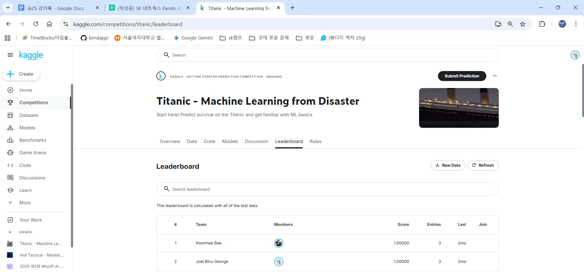
• kaggle은 데이터셋이 고정되어있어서 test_dataset에 과적합시켜버리는 케이스도 많음.

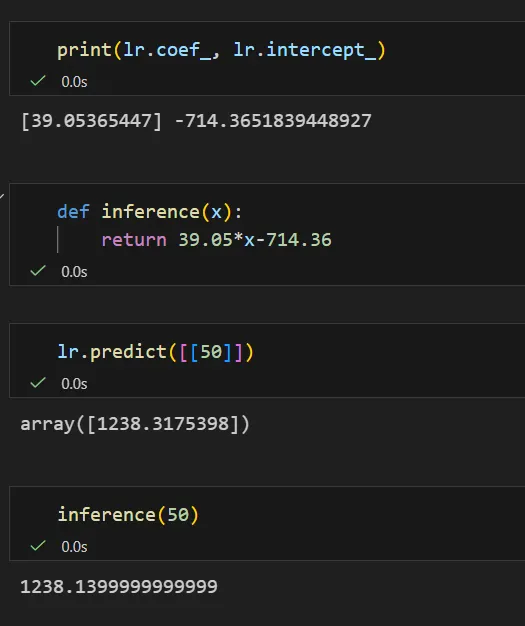
• linear regression에서 가능한 가중치 편향 체크.

Xai → 설명 가능한 인공지능 방법론

🔵단순선형회귀 시각화

import matplotlib.pyplot as plt

plt.scatter(X_train, y_train)
plt.plot(np.arange(60),lr.predict(np.arange(60).reshape(-1,1)),'red')
plt.xlim(-1,55)
plt.show()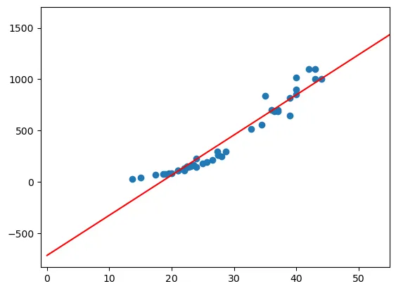

Day2

https://guru.tistory.com/44

🟢정규방정식을 통해 회귀식에 접근해보자~

• 한바탕 지나간 선대 파티
  

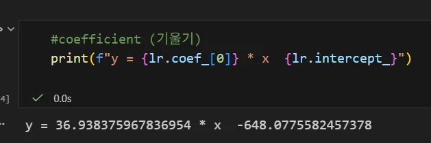
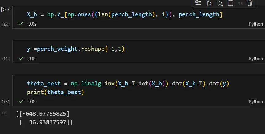
• 정규방정식으로 계수와 절편 도출

DNN 에서는 각 노드가 텐서이다.

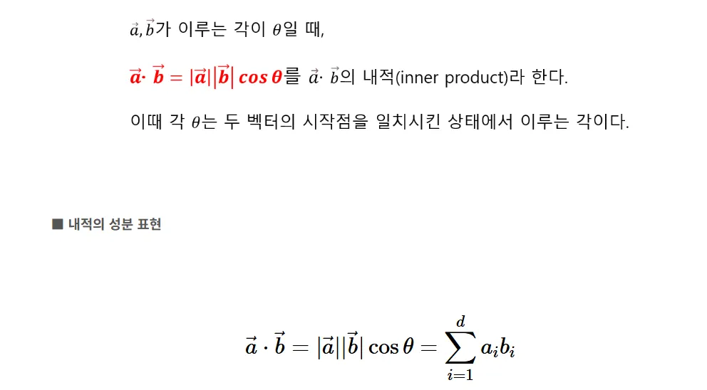
🔵내적

• a의 변화를 벡터 b가 얼마만큼 설명해줄 수 있는가?
• 값이 크면 비슷한 데이터라고 볼 수 있다.

🔵워드임베딩까지 내용이 점프했네….

• 벡터DB에 저장됨.
• PCA, eigen vector, eigen value

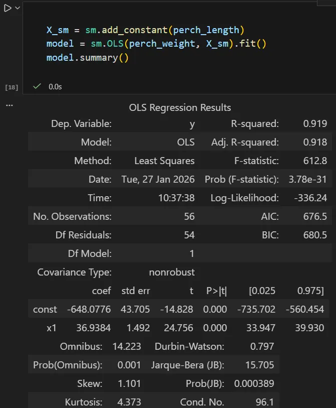
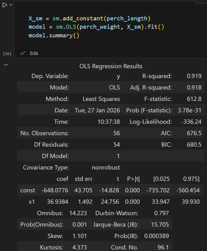
🟢이젠 statsmodel 써볼게

• 변수

  • H0(귀무가설) : 계수가 0이다.
  • H1(대립가설): 계수가 0이 아니다.
  • p-value (0.05) 이하 → 귀무가설을 기각한다.

• F-statistic (F 검정) - 전체 모형에 대한 판단

  • H0(귀무가설) : 모든 계수가 0이다.
  • H1(대립가설) : 하나 이상의 계수는 0이 아니다.

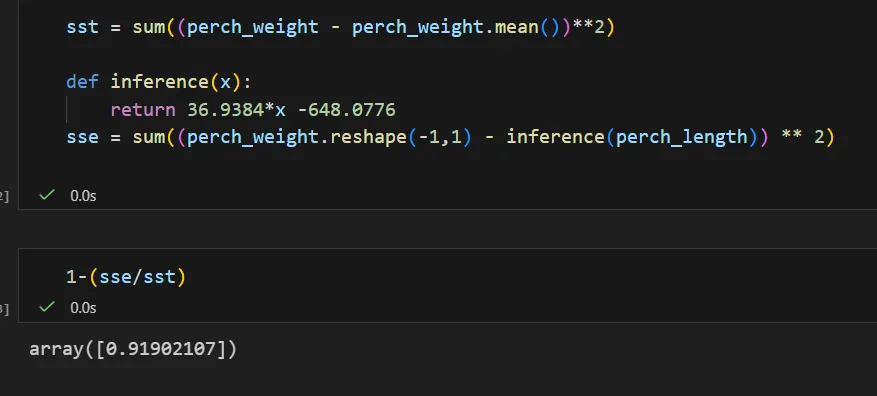
• R-squared

  • 설명력(0~1)

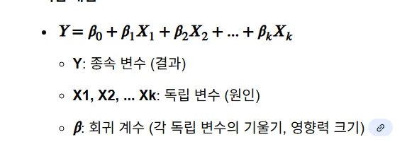
🔵다중 회귀

🟢스케일링

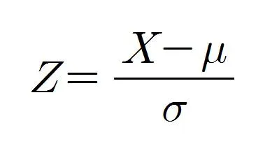
• 표쥰화
• 회귀에서 많이 씀

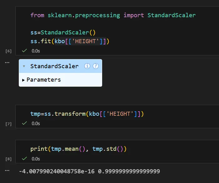
• fit하고, transform

from sklearn.preprocessing import StandardScaler

ss=StandardScaler()
ss.fit_transform(kbo[['HEIGHT']])

• 한 번에 가능

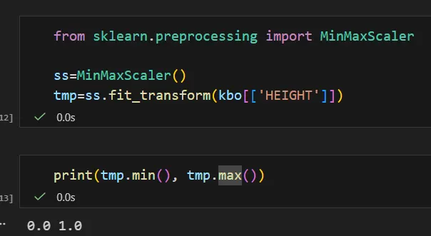
• 정규화

  • 딥러닝에서 많이 쓰임

🔵test와 train을 표준화할 때 올바른 순서는?

from sklearn.preprocessing import StandardScaler
ss=StandardScaler()

train_scaler =ss.fit_transform(train[['HEIGHT']])
test_scaler=ss.transform(test[['HEIGHT']])

• train으로 fit_transform
• test는 train으로 fit한 scaler로 test를 transform

🔵라벨인코더

from sklearn.preprocessing import LabelEncoder
le = LabelEncoder()
le.fit(kbo['TEAM'])
le.classes_
le.transform(kbo['TEAM'])

• 숫자가 클 수록 좋다고 모델이 오해할 수 있음
• 이에 대한 대책 → 원핫 인코더

🔵원핫 인코더

from sklearn.preprocessing import OneHotEncoder
oh = OneHotEncoder(sparse_output=False)
oh.fit(kbo[['TEAM']])
kbo_oh = oh.transform(kbo[['TEAM']])

oh.get_feature_names_out()

array(['TEAMKIA 타이거즈', 'TEAM_KT 위즈', 'TEAM_LG 트윈스', 'TEAM_NC 다이노스',
'TEAM_SSG 랜더스', 'TEAM고양 히어로즈', 'TEAM두산 베어스', 'TEAM롯데 자이언츠',
'TEAM삼성 라이온즈', 'TEAM상무 ', 'TEAM키움 히어로즈', 'TEAM한화 이글스'],
dtype=object)

pd.DataFrame(kbo_oh, columns=oh.get_feature_names_out())

kbo_one_hot = pd.concat([kbo, pd.DataFrame(kbo_oh, columns=oh.get_feature_names_out())] , axis=1)

• 원핫인코딩 적용한 코드로 추가
• 근데 원핫인코딩 같은 경우는 컬럼을 하나 드랍에도 의미 보전에 무리가 없음.

from sklearn.preprocessing import OneHotEncoder
oh = OneHotEncoder(sparse_output=False,drop='first')
oh.fit(kbo[['TEAM']])
kbo_oh = oh.transform(kbo[['TEAM']])

• drop = ‘first’
• drop = ‘if_binary’?
  • 컬럼 수 바뀌지 않음

🔵갑자기 경사하강법

• 이차함수에 learning rate 설정하는 얘기
• 로지스틱 회귀 이야기하다가
• 시그모이드 함수 이야기하다가
• 미분 얘기하다가
• 여기로 넘어왔다.

🟢갑분보스턴

• 집값 예측을 해보아요.

y = boston.pop('MEDV')

import seaborn as sns
import matplotlib.pyplot as plt

fig, axs = plt.subplots(figsize=(16,8), ncols=4, nrows=2)
lm_features = ['ZN', 'INDUS', 'NOX', 'RM', 'AGE', 'RAD',  'PTRATIO',  'LSTAT']
for i, feature in  enumerate(lm_features):
    row = int(i/4)
    col = i%4
    sns.regplot(x=feature, y=y, data=boston, ax=axs[row][col])

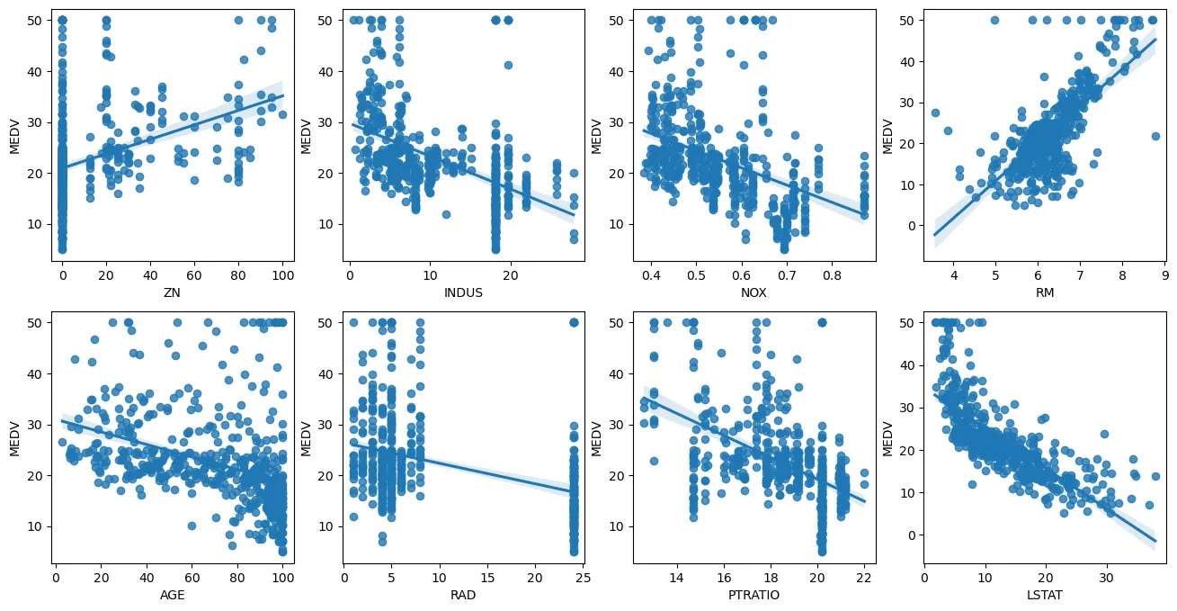
시각적으로 상관관계를 확인하는 코드

boston.corr()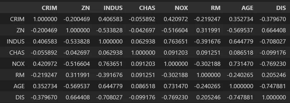

• 통계에서는 상관관계를 본다.

🔵다중공산성

• 통계에서는 독립변수 X는 종속변수 Y하고만 상관관계가 있어야 하며, 독립변수끼리는 상관관계가 있어서는 안된다.

🔵진짜 예측해보자

from sklearn.model_selection import train_test_split

X_train, X_test, y_train, y_test = train_test_split(boston,y, test_size=0.3, random_state=42)

from sklearn.preprocessing import StandardScaler
ss=StandardScaler()

X_train_scaled =ss.fit_transform(X_train)
X_test_scaled=ss.transform(X_test)

• 당연하지만 y는 스케일 하는게 아니다.

from sklearn.linear_model import LinearRegression

lr=LinearRegression()

lr.fit(X_train_scaled,y_train)

lr.coef_

array([-1.10834602, 0.80843998, 0.34313466, 0.81386426, -1.79804295,
2.913858 , -0.29893918, -2.94251148, 2.09419303, -1.44706731,
-2.05232232, 1.02375187, -3.88579002])

lr.intercept_

np.float64(23.01581920903955)

from sklearn.metrics import mean_squared_error, r2_score
r2_score(y_test, lr.predict(X_test_scaled))
mean_squared_error(y_test, lr.predict(X_test_scaled))

21.517444231177212

from sklearn.metrics import mean_squared_error,mean_absolute_error, r2_score

mean_absolute_error(y_test, lr.predict(X_test_scaled))

3.1627098714574053 → mse는 제곱 기준, mae는 절댓값 기준이라 수치가 상대적으로 작음.

from sklearn.metrics import mean_squared_error,mean_absolute_error, r2_score, root_mean_squared_error
#r2_score(y_test, lr.predict(X_test_scaled))
#mean_squared_error(y_test, lr.predict(X_test_scaled))
#mean_absolute_error(y_test, lr.predict(X_test_scaled))

root_mean_squared_error(y_test,lr.predict(X_test_scaled))

4.638689926172821

• mse에 제곱근 씌우기.

from sklearn.metrics import mean_squared_error,mean_absolute_error, r2_score, root_mean_squared_error
r2_score(y_test, lr.predict(X_test_scaled))

0.7112260057484932

• 설명력
• 데이터의 분산을 이 모델이 얼마나 잘 설명하고 있는지 의미함.

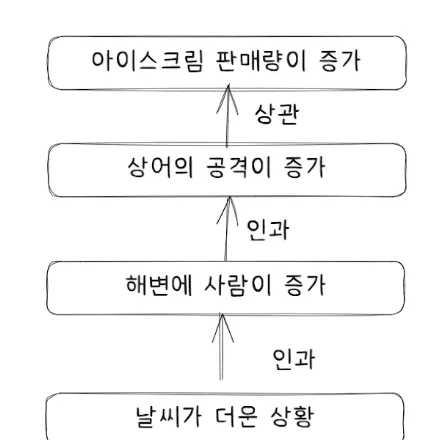
🟢상관관계와 인과관계의 차이

🔵상관관계

• 두 가지 변수 간의 어떤 선형적 관계를 갖고 있는지를 분석하는 통계 기법

🔵인과관계

• 외부 요인을 통제한 상태에서, 두 변수가 원인과 결과의 관계를 맺고 있는지 분석
• 지피티는 인과관계 기반 모델.
• 날씨가 더워서 해변에 사람이 증가 → 상어의 공격이 증가
• → 아이스크림 판매량 증가(상관관계)

+) 모델이 노이즈까지 학습을 하는게 유익할까?

전혀 그러지 않다. 그래서 필요한 것이 규제.

Day3

🟢옥탄가 데이터 기반 통계 공부

🔵 표본 통계값

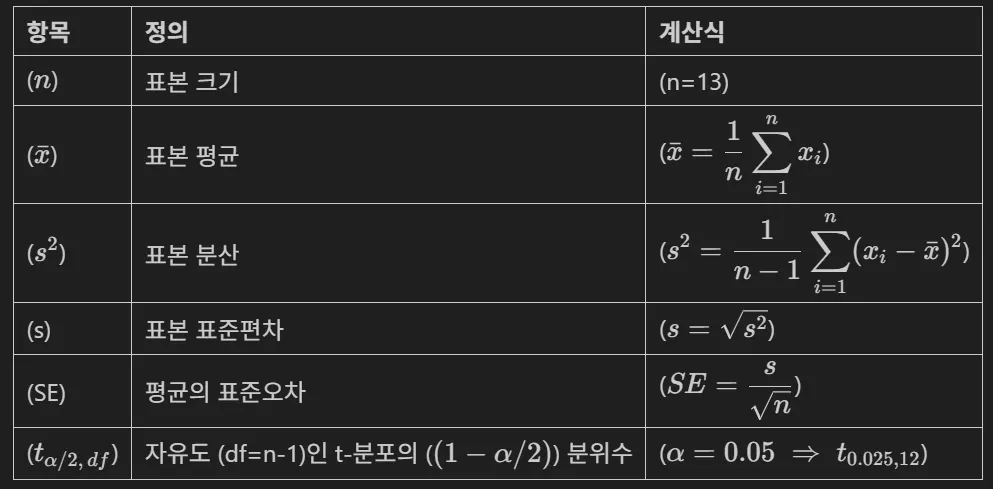
🔵 평균, 표준편차

import numpy as np
from scipy import stats

#샘플
octane=np.array([88.6, 86.4, 87.2, 88.4, 87.2, 87.6, 86.8, 86.1, 87.4, 87.3, 86.4, 86.6, 87.1])

print("평균",np.mean(octane))
print("표준편차 자유도 1" , np.std(octane,ddof=1))
print("표준편차 자유도 0", np.std(octane,ddof=0))

평균 87.16153846153844
표준편차 자유도 1 0.7422246532536062
표준편차 자유도 0 0.7131063806047254

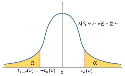
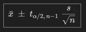
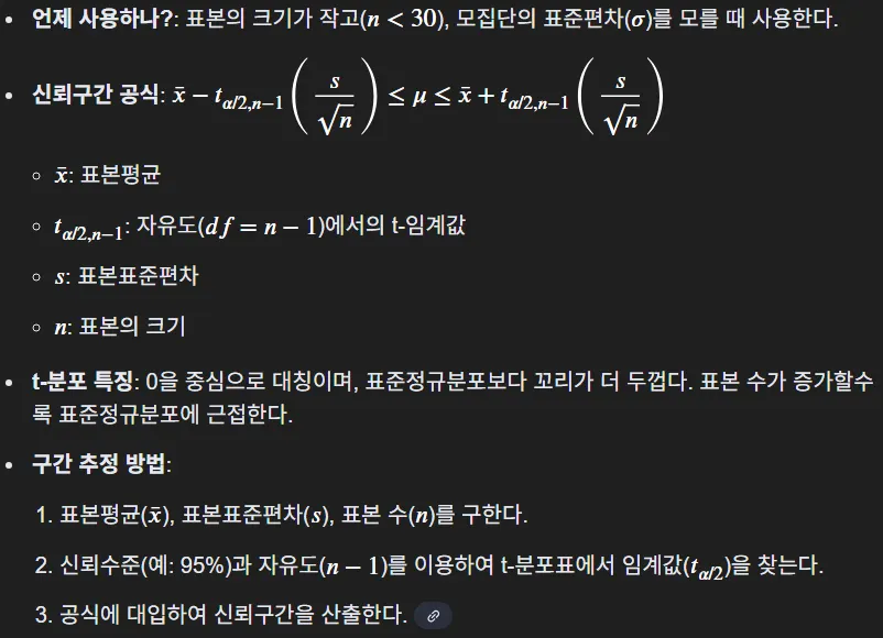
🔵 t분포

import numpy as np 
from scipy import stats

octane = np.array([88.6, 86.4, 87.2, 88.4, 87.2, 87.6, 86.8, 86.1, 87.4, 87.3, 86.4, 86.6, 87.1])

# 샘플 평균 
# 샘플 표준편차 
# 자유도 1를 제거 
n = len(octane)
mean = np.mean(octane)
sd = np.std(octane, ddof=1)

df = n - 1
alpha = 0.05
t_crit = stats.t.ppf( 1 - alpha/2, df)
se = sd  / np.sqrt(n)

margin = t_crit * se
lower = mean - margin 
upper = mean + margin

print(f"신뢰구간 {lower} , {upper}")

신뢰구간 86.71301659249545 , 87.61006033058143

🟢규제(릿지,라쏘)

🔵 릿지

유클라디안 거리

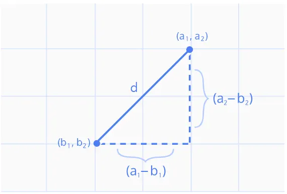
🔵 라쏘

맨해탄 거리

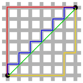
강사님 너무 어려워요

from sklearn.linear_model import LinearRegression, Ridge, Lasso
import pickle
with open("./ml_regssion.pkl", "rb") as f:
    ml = pickle.load(f)

for key, val in ml.items():
    locals()[key] = val

X_train_scaler = scaler.transform(X_train)
import pandas as pd 
pd.DataFrame(X_train_scaler).describe()

X_test_scaler = scaler.transform(X_test)
pd.DataFrame(X_test_scaler).describe()

# Ridge 
ridge = Ridge()
ridge.fit(X_train_scaler, y_train)

lasso = Lasso()
lasso.fit(X_train_scaler, y_train)

from sklearn.metrics import mean_absolute_error, mean_squared_error, root_mean_squared_error
# regression 
print (f"regression --> {model.coef_} , {model.intercept_}")
print (f"model --> {root_mean_squared_error(y_test, model.predict(X_test_scaler))}")

print("-" * 50)
# ridge
print (f"ridge -->  {ridge.coef_} , {ridge.intercept_}")
print (f"ridge --> {root_mean_squared_error(y_test, ridge.predict(X_test_scaler))}")
print("-" * 50)
# lasso
print (f"lasso -> {lasso.coef_} , {lasso.intercept_}")
print (f"{root_mean_squared_error(y_test, lasso.predict(X_test_scaler))}")

regression --> [-1.10834602 0.80843998 0.34313466 0.81386426 -1.79804295 2.913858
-0.29893918 -2.94251148 2.09419303 -1.44706731 -2.05232232 1.02375187
-3.88579002] , 23.01581920903955

model --> 4.6386899261728205

ridge --> [-1.09593334 0.78820029 0.31413846 0.81943277 -1.76159118 2.91992552
-0.30160552 -2.90234902 2.01278255 -1.376115 -2.04111302 1.02096425
-3.87116058] , 23.01581920903955

ridge --> 4.642052735184102

lasso -> [-0. 0. -0. 0.22497382 -0. 2.73102016
-0. -0. -0. -0. -1.24748188 0.26711155
-3.75408325] , 23.01581920903955
5.150968677089682

alphas = [0, 0.1, 1, 10, 100,10000] 
for alpha in alphas:
    lasso = Lasso(alpha=alpha)
    lasso.fit(X_train_scaler, y_train)
    print (f"lasso alpha{alpha} --> {root_mean_squared_error(y_test, lasso.predict(X_test_scaler))}")

lasso alpha0 --> 4.6386899261728285
lasso alpha0.1 --> 4.773725883163098
lasso alpha1 --> 5.150968677089682
lasso alpha10 --> 8.780576101609647
lasso alpha100 --> 8.780576101609647
lasso alpha10000 --> 8.780576101609647

🟢fastapi 기반 모델 서빙

🔵코드

from fastapi import FastAPI
from pydantic import BaseModel
import pickle

app = FastAPI()

class House(BaseModel):
    CRIM : float
    ZN : float
    INDUS : float
    CHAS : float
    NOX : float
    RM : float
    AGE : float
    DIS : float
    RAD : float
    TAX : float
    PTRATIO : float
    B : float
    LSTAT : float
 
with open("./ml_regssion.pkl",'rb') as f:
    ml=pickle.load(f)

model=ml['model']
scaler=ml['scaler']

print("모델이 정상적으로 로드됨")
@app.post('/house_price_predict/')
async def get_post(item : House):
    pass
    

🔵uvicorn

• 가벼운 웹서버. was Server
• 서버는 보통 웹서버가 와스서버 이렇게 두 개 있다.

🔵로드밸런서

• Nginx가 주로 함
• 사람 분산처리해줌

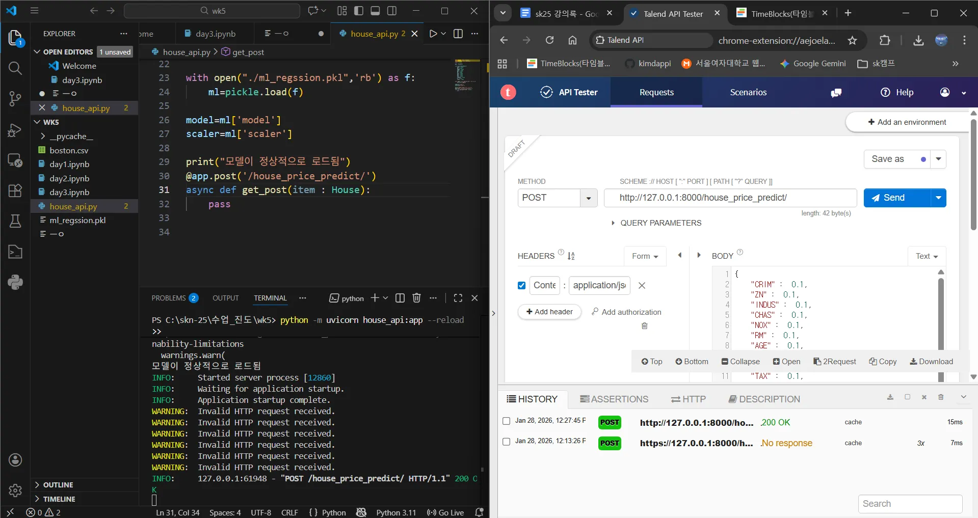
Talend API 확장프로그램 사용

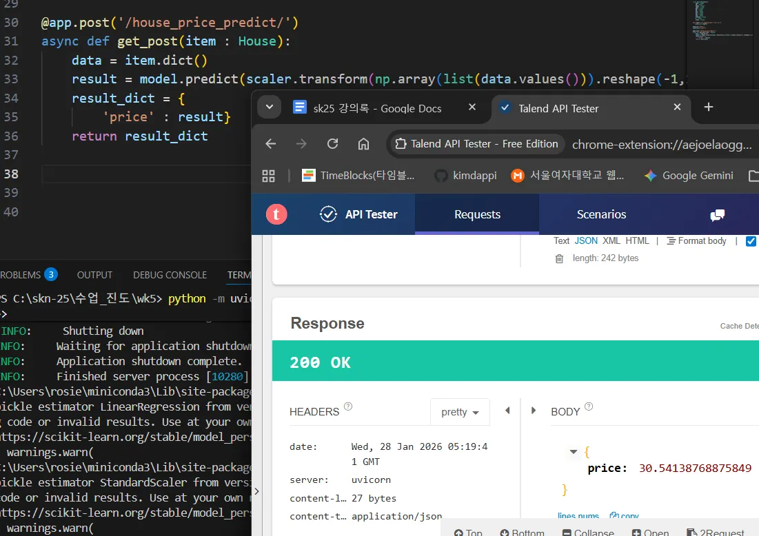
• 코드에서 모델 돌려서 api 확인 사이트에서 body에서 price 확인

celery. redis

챗봇 설계 때 redis 사용 가능

• 카프카 분산처리.

도커 쿠버네티스

import matplotlib.pyplot as plt
import numpy as np

def sigmoid(x):
    return 1   / (1 + np.exp(-x))

x = np.arange(-10, 10, 0.1)
y = sigmoid(x)

plt.figure(figsize=(8,5))
plt.plot(x,y)

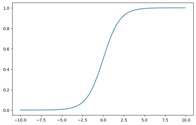
• 임계점이 0.5 언제? x가 0일때
• 오즈비를 통해 시그모이드 함수 유도 가능.

🟢아이리스..

from sklearn.linear_model import LogisticRegression
from sklearn import datasets

iris = datasets.load_iris()

iris_df = pd.DataFrame(iris['data'], columns=iris['feature_names'])

iris_df_2 = iris_df[(iris['target'] == 0) | (iris['target'] == 1)].copy()

y = iris['target'][:100]

from sklearn.model_selection import train_test_split

X_train, X_test, y_train, y_test =train_test_split(iris_df_2,y,test_size=0.2,random_state=42, stratify=y)
# stratify를 통해 y 클래스 불균형을 피함

np.unique(y_train, return_counts=True)

(array([0, 1]), array([40, 40]))

logit=LogisticRegression()
logit.fit(X_train,y_train)

logit.predict(X_test)==y_test

from sklearn.metrics import confusion_matrix

confusion_matrix(y_test, logit.predict(X_test))

array([[10, 0],
[ 0, 10]])

Day4

🟢분류 성능 평가 - 혼동행렬 기반

🔵개념 정리

이진분류 태스크

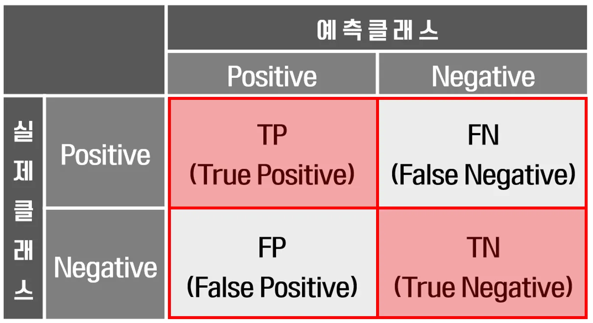
• accuracy : TP+TN /네 칸 전부 ⇒ 분자 모두 진실.
• precision : TP / (TP+FP)
  • 주식 태스크
  • 스팸 메일 → 스팸이 아닌 중요한 메일을 스팸으로 오인하면 업무에 큰 지장이 생김
• Recall, sensivity : TP/(TP+FN) → 환자 관련 테스크
  • 병원, 암진단, 금융 사기 → 실제 환자 놓치면 치명적, 후처리하면 됨.
• specificity : TN/(FP+TN) →실제 음성인 데이터 중 모델이 음성이라고 맞게 예측한 값

precision - recall ⇒ Trade-off

• F1 score → Precision, Recall의 조화 평균.

  • 2 (precision recall)/(precision+recall)

• 위양성률(False Positive Rate) : 실제 음성인데 모델이 양성이라고 잘못 판단한 것

  • ex) 오진
  • FP/(TN+FP)

• ROC

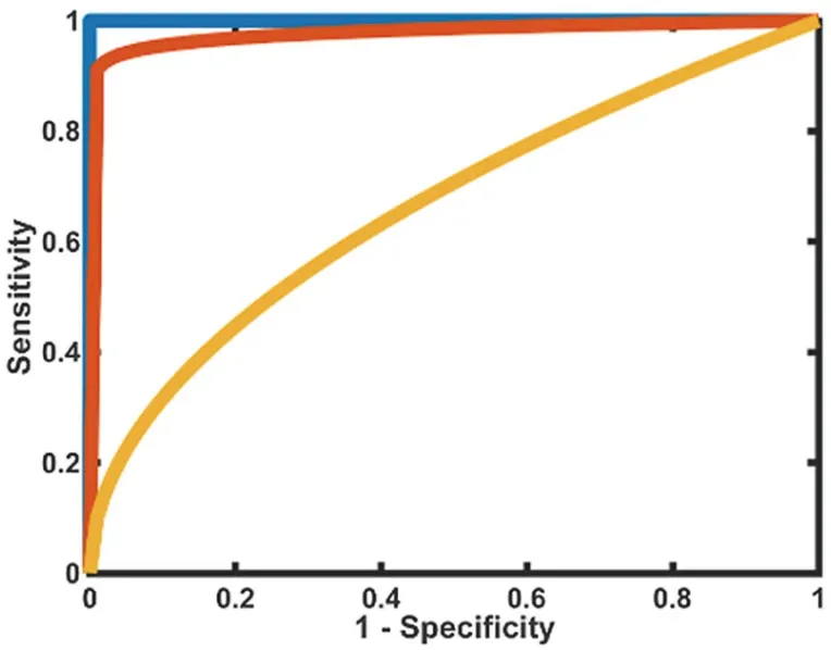
파란색 빨간색 노란색 순으로 좋음

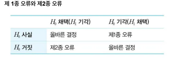
• 제 1종 오류 : 남성에게 임신했다고 진단(FP)
• 제 2종 오류 : 임신한 여성에게 임신하지 않았다고 진단(FN)
  • 더 심각한 오류라고 볼 수 있음.

🟢타이타닉 데이터 기반 분석

import pandas as pd
import seaborn as sns

titianic_df= pd.read_csv("titanic_train.csv")

titianic_df.info() 

• passengerid 없어도 된다고 판단

titianic_df.drop(columns='PassengerId',inplace=True)

titianic_df['Survived'].value_counts(normalize=True)

Survived
0 0.616162
1 0.383838
Name: proportion, dtype: float64

🔵손실함수

• 분류 테스크를 수행하기 위해 필요
• 모델이 판단하기 위한 지도.
• 각 모델마다 손실함수는 다르다.

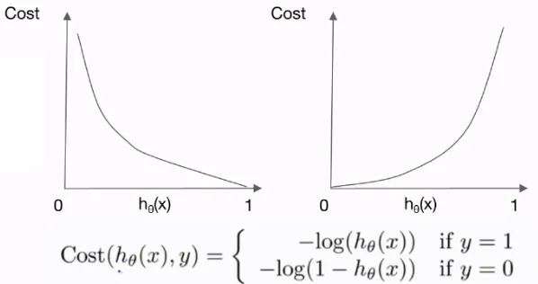
🔵로지스틱 회귀 손실함수

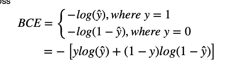
🔵 바이너리 크로스 엔트로피

• 로지스틱 회귀 손실함수와 비슷하게 y값에 따라 식이 다름

• 원빈과 차은우 - 엔트로피가 낮음

• 차은우 옥동자 - 엔트로피가 높음

⇒ 엔트로피는 정보값이라고 볼 수 있다.

로지스틱 회귀에서 엔트로피 값이 크면 오답을 예측하고 있다고 볼 수 있음

titianic_df.describe(include='all')

	Survived	Pclass	Name	Sex	Age	SibSp	Parch	Ticket	Fare	Cabin	Embarked
count	891.000000	891.000000	891	891	714.000000	891.000000	891.000000	891	891.000000	204	889
unique	NaN	NaN	891	2	NaN	NaN	NaN	681	NaN	147	3
top	NaN	NaN	Braund, Mr. Owen Harris	male	NaN	NaN	NaN	347082	NaN	G6	S
freq	NaN	NaN	1	577	NaN	NaN	NaN	7	NaN	4	644
mean	0.383838	2.308642	NaN	NaN	29.699118	0.523008	0.381594	NaN	32.204208	NaN	NaN
std	0.486592	0.836071	NaN	NaN	14.526497	1.102743	0.806057	NaN	49.693429	NaN	NaN
min	0.000000	1.000000	NaN	NaN	0.420000	0.000000	0.000000	NaN	0.000000	NaN	NaN
25%	0.000000	2.000000	NaN	NaN	20.125000	0.000000	0.000000	NaN	7.910400	NaN	NaN
50%	0.000000	3.000000	NaN	NaN	28.000000	0.000000	0.000000	NaN	14.454200	NaN	NaN
75%	1.000000	3.000000	NaN	NaN	38.000000	1.000000	0.000000	NaN	31.000000	NaN	NaN
max	1.000000	3.000000	NaN	NaN	80.000000	8.000000	6.000000	NaN	512.329200	NaN	NaN

from sklearn.preprocessing import OneHotEncoder
oh = OneHotEncoder(sparse_output=False)
oh.fit(kbo[['TEAM']])
kbo_oh = oh.transform(kbo[['TEAM']])
oh.get_feature_names_out()

pd.DataFrame(kbo_oh, columns=oh.get_feature_names_out())

kbo_one_hot = pd.concat([kbo, pd.DataFrame(kbo_oh, columns=oh.get_feature_names_out())] , axis=1)

• 갑자기 원핫인코딩 더하는 법 까먹어서 넣어봄

import matplotlib.pyplot as plt

plt.style.use("ggplot")

titanic_df = pd.read_csv("./titanic_train.csv")

titanic_df.describe()
titanic_df.describe(include=['O'])

# titanic_df.info()
titanic_df.drop(['PassengerId'], axis=1, inplace=True)

titanic_df['Survived'].value_counts(normalize=True)

titanic_df.isnull().sum()

import matplotlib.pyplot as plt
plt.style.use('ggplot')

titanic_df.groupby(['Embarked', 'Survived'])[['Survived']].count().rename(columns={'Survived' : 'Count'})

embarked = titanic_df.groupby(['Embarked', 'Survived'])[['Survived']].count().rename(columns={'Survived' : 'Count'}).unstack()

embarked.plot.bar()
plt.show()

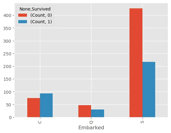
• EDA……………란 시각화…?

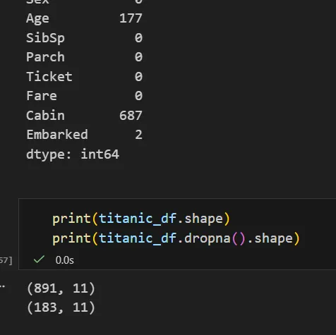
• dropna를 통해 결측치 제거 시 너무 많은 데이터가 손실될 수 있으므로 유의해야한다.

# 기본 dropna
# 하나라도 NaN이 있으면 해당 행 삭제 (axis=0, how='any'가 기본값)
df.dropna()

# Age 컬럼 결측치만 기준으로 행 삭제
# Age가 NaN인 행만 제거, 다른 컬럼 NaN은 무시
df.dropna(subset=['Age'])

# 여러 컬럼을 기준으로 결측치 처리
# Age 또는 Gender 중 하나라도 NaN이면 삭제
df.dropna(subset=['Age', 'Gender'], how='any')

# 여러 컬럼이 모두 NaN일 때만 삭제
# Age와 Gender가 둘 다 NaN인 행만 제거
df.dropna(subset=['Age', 'Gender'], how='all')

# thresh 사용
# NaN이 아닌 값이 최소 8개 이상인 행만 유지
df.dropna(thresh=8)

# subset + thresh 조합
# A, B, C, D 중 NaN이 아닌 값이 3개 이상인 행만 유지
df.dropna(subset=['A', 'B', 'C', 'D'], thresh=3)

# 열(column) 기준으로 결측치 처리
# 하나라도 NaN이 있는 컬럼 삭제
df.dropna(axis=1)

# 열 기준 + thresh
# 값이 500개 이상 존재하는 컬럼만 유지
df.dropna(axis=1, thresh=500)

# 완전히 비어 있는 행만 제거
# 모든 컬럼이 NaN인 행만 삭제
df.dropna(how='all')

• 강의자료 결측치 pdf 같이 봄.

titanic_df.Name.str.split('[,.]',expand=True)

0	1	2	3
0	Braund	Mr	Owen Harris
1	Cumings	Mrs	John Bradley (Florence Briggs Thayer)
2	Heikkinen	Miss	Laina
3	Futrelle	Mrs	Jacques Heath (Lily May Peel)
4	Allen	Mr	William Henry

name_df.drop(columns=3,inplace=True)
name_df.columns = ['last_name', 'honorific', 'first_name']
name_df.map(lambda x:x.strip())
t_df=pd.concat([titanic_df,name_df],axis=1)

import seaborn as sns
plt.figure(figsize=(18,5))
sns.boxplot(data=t_df,x='honorific',y='Age')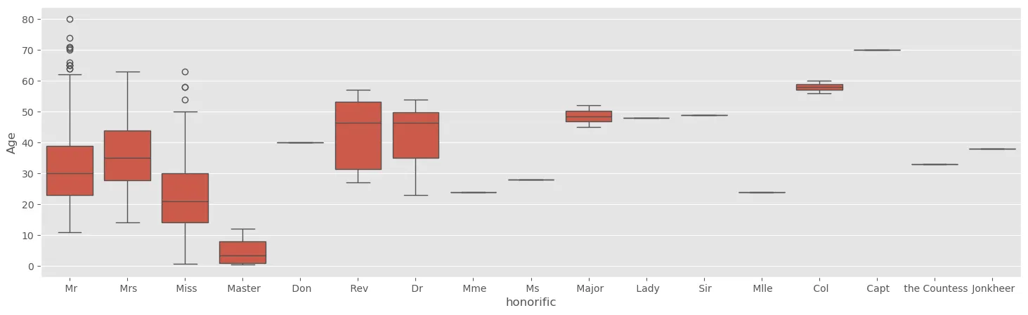

import seaborn as sns
plt.figure(figsize=(18,5))
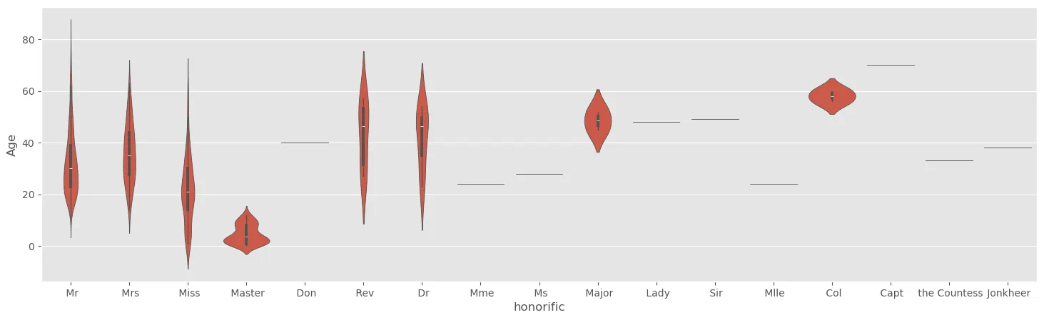
sns.violinplot(data=t_df,x='honorific',y='Age')

• 커널 밀도 추정 (Kernel Density Estimation) 기반

🟢배경지식

쿠버네티스 .

오케스트레이션.

MSA

모놀리식 아키텍처와 마이크로 서비스 아키텍처 비교

마이크로 서비스 아키텍처 - 컨테이너 기술이 있는지 없는지?

scale out autoscaling

random_seed = 42?

은하수를 여행하는 히치하이커를 위한 안내서

🟢타이타닉 모델링

titanic_df = pd.read_csv("./titanic_train.csv")

titanic_df.describe()
titanic_df.describe(include=['O'])

# titanic_df.info()
titanic_df.drop(['PassengerId'], axis=1, inplace=True)

titanic_df['Survived'].value_counts(normalize=True)

name_df=titanic_df.Name.str.split('[,.]',expand=True)

name_df.drop(columns=3,inplace=True)

name_df.columns = ['last_name', 'honorific', 'first_name']

name_df.map(lambda x:x.strip())
t_df=pd.concat([titanic_df,name_df],axis=1)

honorific_age = t_df.groupby(['honorific'], as_index=False)[['Age']].mean()

pd.merge(t_df, honorific_age, left_on='honorific', right_on='honorific', how='inner')

t_df_2 = pd.merge(t_df, honorific_age, left_on='honorific', right_on='honorific', how='inner')

t_df_2.loc[t_df_2.Age_x.isnull(), 'Age_x'] = t_df_2.loc[t_df_2.Age_x.isnull(), 'Age_y']

t_df_2.isnull().sum()

t_df_2.drop(['first_name', 'Age_y'], axis=1, inplace=True)

t_df_2.loc[~t_df_2.honorific.isin(['Mr' , 'Miss' , 'Mrs', 'Master']), 'honorific'] = 'other'

t_df_2.drop(['Name', 'Ticket', 'last_name'], axis=1, inplace=True)

t_df_2.drop('Cabin', axis=1, inplace=True)

t_df_2.dropna(inplace=True)

t_df_2.reset_index(drop=True, inplace=True)

from sklearn.preprocessing import OneHotEncoder

en = OneHotEncoder(sparse_output=False, drop='first')

dataset = pd.concat([t_df_2, pd.DataFrame(en.fit_transform(t_df_2[['Sex']] ), columns=en.get_feature_names_out())],axis=1).drop('Sex', axis=1)

from sklearn.preprocessing import LabelEncoder
le =LabelEncoder()

le.fit_transform(dataset[['Embarked']])

from sklearn.preprocessing import OrdinalEncoder
import pandas as pd
oe = OrdinalEncoder(categories=[['S', 'Q', 'C']])

dataset = pd.concat([dataset, pd.DataFrame(oe.fit_transform(dataset[['Embarked']]))], \
          axis=1).drop('Embarked', axis=1).\
    rename(columns={0 : 'Embarked'})

Oe = OneHotEncoder(sparse_output=False, drop='first')
hono_one_hot = pd.DataFrame(Oe.fit_transform(dataset[['honorific']]), columns= Oe.get_feature_names_out())

dataset = pd.concat([dataset, hono_one_hot] ,axis=1).drop('honorific', axis=1)

Y = dataset.pop('Survived')

from sklearn.model_selection import train_test_split

X_train,X_test,y_train,y_test = train_test_split(dataset,Y,random_state=42, test_size= 0.2)

https://dhpark1212.tistory.com/entry/RestAPI-FastAPI-Flask-%EC%B0%A8%EC%9D%B4

lr.fit(X_train_scaler, y_train)
from sklearn.metrics import accuracy_score, recall_score, precision_score, confusion_matrix, f1_score, classification_report

accuracy_score(y_test, lr.predict(ss.transform(X_test)))
confusion_matrix(y_test, lr.predict(ss.transform(X_test)))
print(classification_report(y_test, lr.predict(ss.transform(X_test))))

precision    recall  f1-score   support

           0       0.82      0.88      0.85       110
           1       0.78      0.69      0.73        68

    accuracy                           0.81       178
   macro avg       0.80      0.79      0.79       178
weighted avg       0.81      0.81      0.81       178

• 결론 : 어떤 업무를 수행할 것인지에 따라서 목표 성능지표가 다르다.

lr.predict_proba(ss.transform(X_test))#[:,1]

array([[0.94959902, 0.05040098],
[0.89732007, 0.10267993],
[0.89732007, 0.10267993],
[0.90248374, 0.09751626],
[0.92670505, 0.07329495],

• 가로로 더하면 1
• 확률 기준 지금의 threshold = 0.5

pd.DataFrame(results, columns=['thres', 'acc', 'prec' , 'recall'])

precisions, recalls, thresholds = precision_recall_curve(y_test, pred_proba)

plt.figure(figsize=(8,6))
plt.plot(thresholds, precisions[:len(thresholds)], label = 'Precision')

Day5

🟢이진분류 성능지표

🔵ROC

https://angeloyeo.github.io/2020/08/05/ROC.html

🔵AUC

https://developers.google.com/machine-learning/crash-course/classification/roc-and-auc?hl=ko

🔵트리에서 선택 가능한 성능 지표

지니계수

• 1에 가까울 수록 불평등함을 의미함
• 국가별로 지니계수를 확인할 수 있다.
• 경제학에서도 사용한다.

엔트로피

두 값 모두 작아지는 방향으로 모델을 설계한다.

🟢교차검증

🔵성능 관점

https://bbdata.tistory.com/10

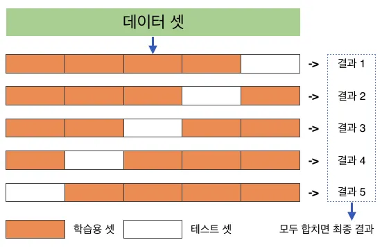
• 사이킷런 - 성능의 평균값
  • 교차 돌려서 제일 성능 좋았을 때의 하이퍼파라미터도 알 수 있음

🔵하이퍼파라미터 관점

• random search
• grid search
• 베이지안 방식 → optuna
  • 하이퍼파라미터가 있음직한 부분에 먼저 찾으러 감

🟢도커

• wsl 켜기

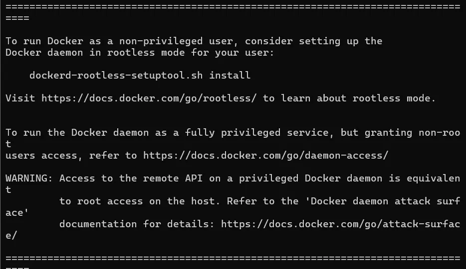
curl -sSL get.docker.com | sh

• 비밀번호 입력 후 기다리기

• 컨테이너 - 가상 공간. 각각의 분리된 공간.
• 도커 - 쿠버네티스 - 마이크로 서비스와 연결됨
• 쿠버네티스에서는 도커를 안쓰고 보통 dll 사용
• 도커는 이미지 개념이 중요

도커 daemon으로 켜졌는지 확인

rosie@ming9:~$ sudo service docker status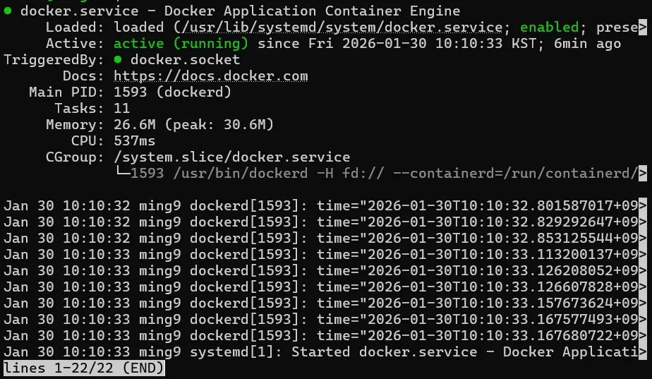

컨테이너 안으로 들어오기

rosie@ming9:~$ sudo docker run -it ubuntu:22.04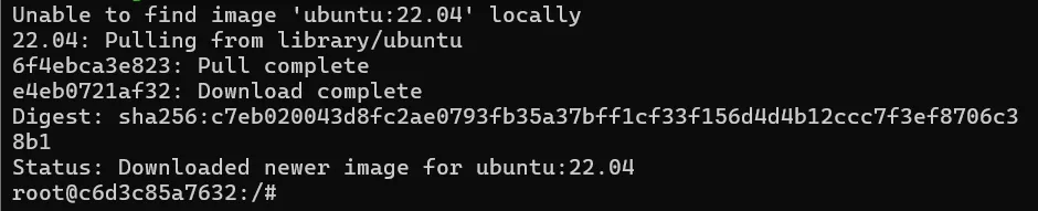

나가기

root@c6d3c85a7632:/# exit

도커 리스트 확인

rosie@ming9:~$ sudo docker ps -a

docker hub

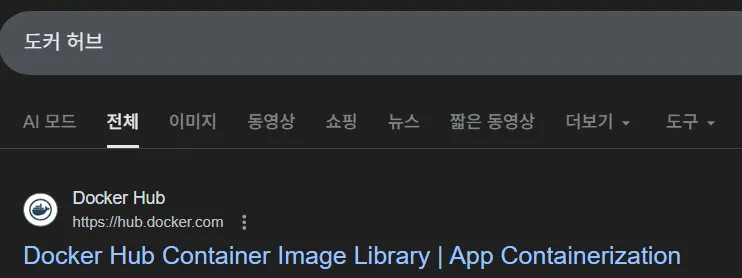
• 이미지 공유하는 곳

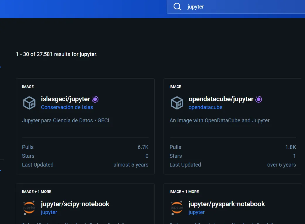
• 사람들이 만들어놓은걸 사용할 수 있음

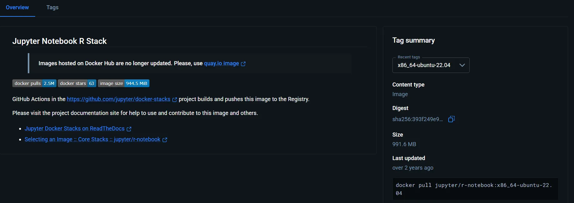
sudo docker pull jupyter/r-notebook:x86_64-ubuntu-22.04

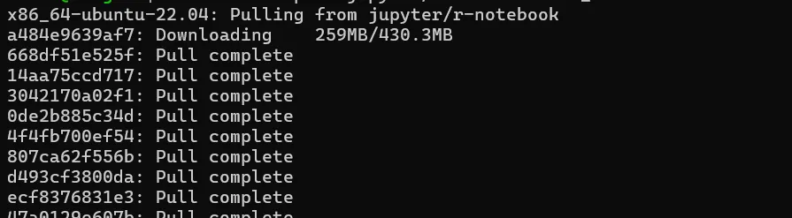
• 이미지 받기
• 명령어 앞에 sudo 포함

다운로드 받아둔 거 확인하기

sudo docker images

이미지 기반 실행

sudo docker run -itd --name rjupyter -p 9000:8888 jupyter/r-notebook:x86_64-ubuntu-22.04

살아있는지 확인

rosie@ming9:~$ sudo docker ps

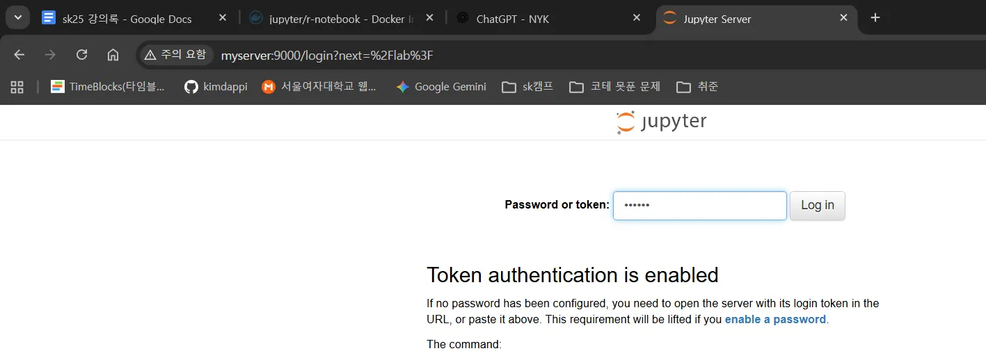
• 주소창에 myserver:9000

비밀번호를 어떻게 아니

rosie@ming9:~$ sudo docker logs rjupyter | grep  http://

token=뒤에있는문자열 윗줄에 넣기

• 분산처리는 scale out
• 포트를 주고받을 수 있어야함.

rosie@ming9:~$ sudo docker ps

rosie@ming9:~$ sudo docker stop rjupyter
rjupyter
rosie@ming9:~$ sudo docker rm rjupyter
rjupyter
rosie@ming9:~$

🔵권한 설정

 sudo usermod -aG docker $USER
 rosie@ming9:~$  sudo usermod -aG docker $USER
[sudo] password for rosie:
rosie@ming9:~$ exit
logout

rosie@ming9:~$ docker ps

docker run -itd --name rjupyter -p 9000:8888 -v ./mydata:/work jupyter/r-notebook:x86_64-ubuntu-22.04

rosie@ming9:~$  sudo chown rosie:rosie ./mydata

rosie@ming9:~$ ls -al |grep mydata

C:\Users\rosie>wsl
rosie@ming9:~$ whoami
rosie
rosie@ming9:~$ pwd
/home/rosie
rosie@ming9:~$ docker ps -aq | xargs -r docker stop
docker ps -aq | xargs -r docker rm
939b71e94aad
939b71e94aad
rosie@ming9:~$ docker ps -a
CONTAINER ID   IMAGE     COMMAND   CREATED   STATUS    PORTS     NAMES
rosie@ming9:~$ mkdir -p /home/rosie/mydata
rosie@ming9:~$ sudo chown -R rosie:rosie /home/rosie/mydata
[sudo] password for rosie:
rosie@ming9:~$ ls -al /home/rosie | grep mydata
drwxr-xr-x  2 rosie rosie     4096 Jan 30 12:06 mydata
rosie@ming9:~$ sudo usermod -aG docker rosie
rosie@ming9:~$ newgrp docker
rosie@ming9:~$ docker ps
CONTAINER ID   IMAGE     COMMAND   CREATED   STATUS    PORTS     NAMES
rosie@ming9:~$ docker run -itd \
  --name rjupyter \
  -p 9000:8888 \
  -v /home/rosie/mydata:/home/jovyan/work \
  jupyter/r-notebook:x86_64-ubuntu-22.04
fae51cc71eadd159ccbd64ee9286b9a4a5e545b8af758ca827adfac10ccd75bd
rosie@ming9:~$ docker logs rjupyter | grep http
https://jupyter-notebook.readthedocs.io/en/latest/migrate_to_notebook7.html
[I 2026-01-30 03:07:02.891 ServerApp] http://fae51cc71ead:8888/lab?token=000042c308d04ed082917345a99216abfebb2485fa305cad
[I 2026-01-30 03:07:02.891 ServerApp]     http://127.0.0.1:8888/lab?token=000042c308d04ed082917345a99216abfebb2485fa305cad
        http://fae51cc71ead:8888/lab?token=000042c308d04ed082917345a99216abfebb2485fa305cad
        http://127.0.0.1:8888/lab?token=000042c308d04ed082917345a99216abfebb2485fa305cad
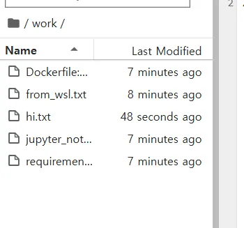
rosie@ming9:~$ touch /home/rosie/mydata/from_wsl.txt

• 마침내 연결
• 파일 탐색기에서 접근할 때는 work/ 안의 수정사항이 보임
  

🔵도커 빌드하기.

리눅스 안에 폴더 하나 임의로 생성(encore)

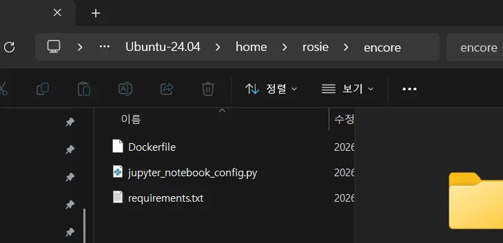
rosie@ming9:~$ pwd
/home/rosie
rosie@ming9:~$ cd encore
rosie@ming9:~/encore$ docker build -t sk25:0.1 .
[+] Building 134.8s (9/12)        

확인하기

rosie@ming9:~/encore$ docker images

9000번대 2개 쓰려니 꼬였다

rosie@ming9:~/encore$docker rm rjupyter

rosie@ming9:~/encore$ docker rm sk25

rosie@ming9:~/encore$ docker run -itd \
  --name sk25 \
  -p 9000:8888 \
  -v ~/mydata:/home/ict/work \
  sk25:0.1

• 이제 도커 안에서 주피터랩이 실행된다.

🟢교차검증

🔵단순한 교차검증 코드

from sklearn.model_selection import KFold
from sklearn.datasets import load_iris
import pandas as pd 

iris = load_iris()

df = pd.DataFrame(data=iris['data'],  columns=iris['feature_names'])

kfold = KFold(n_splits=5)

from sklearn.tree import DecisionTreeClassifier
from sklearn.metrics import accuracy_score
total = [] 
for train_index, test_index in kfold.split(df):
    dt = DecisionTreeClassifier()
    # print(f"train_index -> {train_index}")

    # print("-" * 50)
    # print(f"test_index -> {test_index}")
    print("="*50)
    dt.fit(df.iloc[train_index], iris.target[train_index])
    pred = dt.predict( df.iloc[test_index])
    acc = accuracy_score(iris.target[test_index], pred)
    print(f"{acc}")
    total.append(acc)

🔵from sklearn.model_selection import StratifiedKFold

• y값의 클래스 균형 해결

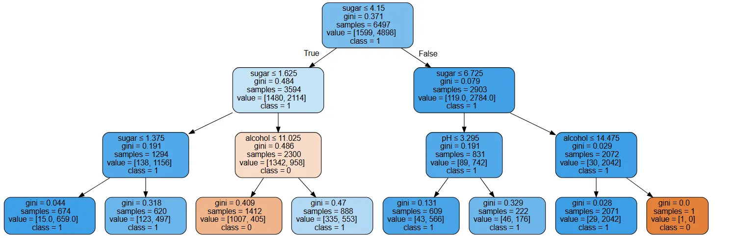
🟢이진트리 - Decision tree

from sklearn.tree import DecisionTreeClassifier, export_graphviz
dataset = pd.read_csv("https://bit.ly/wine_csv_data")

• 이중분류 가능
• 다중분류도 가능하다
• softmax 함수로 나눔

y=dataset.pop('class')
dt = DecisionTreeClassifier(max_depth =3)
dt.fit(dataset,y)

• 과적합 방지를 위해 노드 최대길이 제한

🔵Decision tree 시각화

import graphviz

dot_data = export_graphviz(dt,  out_file=None,  feature_names=['alcohol', 'sugar', 'pH'], 
                class_names = ['0', '1'],
                filled=True,  rounded=True, special_characters=True)

graphviz.Source(dot_data)

🟢앙상블 모델

🔵 random forest

• decision tree 모델을 여러 개 비치한 모델

🔵 voting

• soft voting
  • 확률 평균낸 확률 ⇒ 통상적으로 투표
• hard voting
  • 진짜 투표

🔵 boosting

• 앞에서 예측한 분류기가 틀린 부분에 있어 가중치를 부여한다.
• 제일 대표적인 모델 - xgboost
• 캐글에서 대회에서 많이 사용함. 성능이 아주 좋다기보다 0.0001이라도 높일 수 있음