[밑바닥부터 시작하는 딥러닝] CH5

kimgaeul02·2023년 1월 28일

본 포스팅은 '밑바닥 부터 시작하는 딥러닝' 교재로 공부한 것을 정리했습니다.

CH5. 오차역전법

가중치 매개변수의 기울기를 효율적으로 계산하는 방법으로 수식과 계산 그래프를 통해 이해할 수 있다.

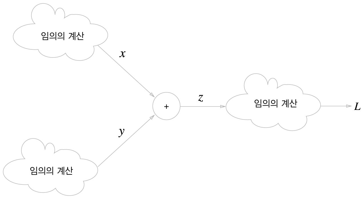
5.1 계산 그래프

계산 과정을 그래프 자료구조로 나타낸 것으로, 복수의 노드(node)와 에지(edge)로 표현된다.

5.1.1 계산 그래프로 풀다

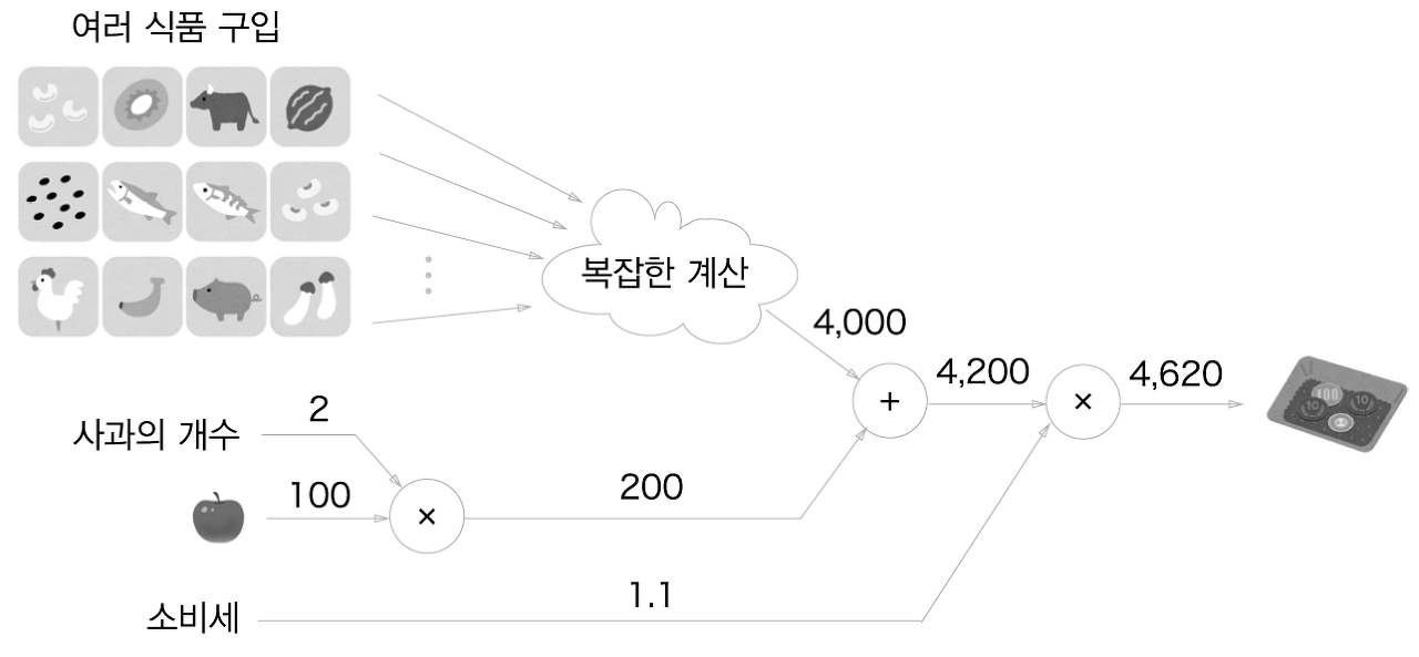
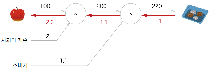
문제 1 : 현빈 군은 슈퍼에서 1개에 100원인 사과를 2개 샀습니다. 이때 지불 금액을 구하세요.단, 소비세가 10% 부과됩니다.
문제 2: 현빈 군은 슈퍼에서 사과를 2개, 귤을 3개 샀습니다. 사과는 1개 100원, 귤은 1개에 150원입니다. 소비세가 10%일 때 지불 금액을 구하세요.

계산 그래프를 이용한 문제풀이는 다음 흐름으로 진행 된다.

계산 그래프를 구성한다.
그래프에서 계산을 왼쪽에서 오른쪽으로 진행한다.

순전파 : 계산 그래프의 출발점부터 종착점으로의 전파이다.
역전파 : 종착점부터 출발점으로의 전파, 미분 계산 시 중요한 역할을 한다.

5.1.2 국소적 계산

계산 그래프의 특징은 '국소적 계산'을 전파함으로써 최종 결과를 얻는다는 점에 있다.
국소적 계산은 전체에서 어떤 일이 벌어지든 상관없이 자신과 관계된 정보만으로 결과를 출력할 수 있다.
단순하지만, 그 결과를 전달함으로써 전체를 구성하는 복잡한 계산을 해낼 수 있다.

5.1.3 왜 계산 그래프로 푸는가?

국소적 계산이 가능하다.
중간 계산 결과를 모두 보관할 수 있다.
역전파를 통해 '미분'을 효율적으로 계산할 수 있다.

5.2 연쇄법칙

국소적 미분을 전달하는 원리는 연쇄법칙(chain rule)을 따른 것이다.

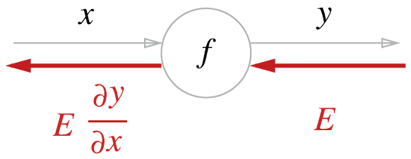
5.2.1 계산 그래프의 역전파

역전파 $y=f(x)$ 의 계산 절차

역전파의 계산 절차는 신호 $E$ 에 노드의 국소적 미분( $\frac{\partial y}{\partial x}$ )을 곱한 후 다음 노드로 전달하는 것이다.
국소적 미분 = 순전파에서 $y=f(x)$ 계산의 미분을 구함 = $x$ 에 대한 $y$ 의 미분 $\frac{\partial y}{\partial x}$ 를 구함
국소적 미분을 상류에서 전달된 값( $E$ )에 곱하여 앞쪽으로 전달하는 것이다.
연쇄법칙의 원리로 설명할 수 있다.

5.2.2 연쇄법칙이란?

합성 함수 : 여러 함수로 구성된 함수
연쇄법칙은 합성 함수의 미분에 대한 성질이며, '합성 함수의 미분은 합성 함수를 구성하는 각 함수의 미분의 곱으로 나타낼 수 있다.' 라고 정의된다.
$z=(x+y)^2$ 라고 가정하였을 때, 연쇄법칙을 이용한 풀이는 다음과 같다.

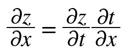
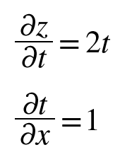
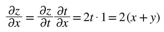
5.2.3 연쇄법칙과 계산 그래프

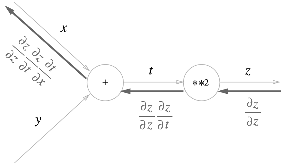
5.3 역전파

5.3.1 덧셈 노드의 역전파

ex) $z=x+y$ 의 미분은 다음과 같이 계산할 수 있다.
$\frac{\partial z}{\partial x}=1$ , $\frac{\partial z}{\partial y}=1$
$\frac{\partial z}{\partial x}$ 와 $\frac{\partial z}{\partial y}$ 모두 1이 된다. 계산 그래프는 다음과 같다.
덧셈 노드의 역전파는 입력 값을 그대로 흘려보낸다.
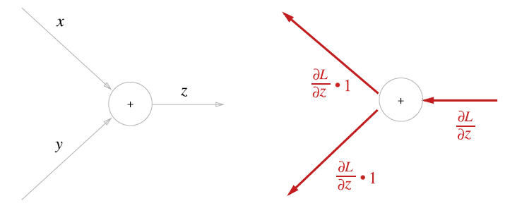
덧셈 노드의 역전파는 1을 곱하기만 할 뿐이므로 입력된 값을 그대로 다음 노드로 보내게 된다.
상류에서 전해진 미분 값을 $\frac{\partial L}{\partial z}$ 라고 한 것은, 최종적으로 $L$ 이라는 커다란 값을 출력하는 큰 계산 그래프를 가정하기 때문이다.

5.3.2 곱셈 노드의 역전파

ex) $z=xy$ 의 미분은 다음과 같이 계산할 수 있다.
$\frac{\partial z}{\partial x}=y$ , $\frac{\partial z}{\partial y}=x$
곱셈 노드 역전파는 상류의 값에 순전파 때의 입력 신호들을 '서로 바꾼 값'을 곱해서 하류로 보낸다.
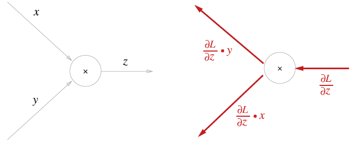
덧셈의 역전파와 달리 순방향 입력 신호 값이 필요하다. 따라서 순전파의 입력 신호를 변수에 저장해둔다.

5.4 단순한 계층 구현하기

사과 쇼핑을 파이썬으로 구현
덧셈 노드는 'AddLayer', 곱셈 노드는 'MulLayer'

5.4.1 곱셈 계층

곱셈 계층 구현

class MulLayer:
  def __init__(self):
    self.x = None
    self.y = None
 
  def forward(self, x, y): #순전파
    self.x = x
    self.y = y
    out = x * y
 
    return out
 
  def backward(self, dout): #역전파
    dx = dout * self.y 
    dy = dout * self.x
 
    return dx, dy

사과 쇼핑 구현

apple = 100
apple_num = 2
tax = 1.1
 
# 계층들
mul_apple_layer = MulLayer()
mul_tax_layer = MulLayer()
 
# 순전파
apple_price = mul_apple_layer.forward(apple, apple_num)
price = mul_tax_layer.forward(apple_price, tax)
 
print(price) 
>>> 220.00000000000003

# 각 변수에 대한 미분
dprice = 1
dapple_price, dtax = mul_tax_layer.backward(dprice)
dapple, dapple_num = mul_apple_layer.backward(dapple_price)
 
print(dapple, dapple_num, dtax)
>>> 2.2 110.00000000000001 200

5.4.2 덧셈 계층

덧셈 계층 구현

class AddLayer:
  def __init__(self):
    pass #초기화 필요 없음
 
  def forward(self, x, y):
    out = x + y
    return out
 
  def backward(self, dout):
    dx = dout * 1
    dy = dout * 1
    return dx, dy

사과 쇼핑 구현

apple = 100
apple_num = 2
orange = 150
orange_num = 3
tax = 1.1
 
# 계층들
mul_apple_layer = MulLayer()
mul_orange_layer = MulLayer()
add_apple_orange_layer = AddLayer()
mul_tax_layer = MulLayer()
 
# 순전파
apple_price = mul_apple_layer.forward(apple, apple_num)  # (1)
orange_price = mul_orange_layer.forward(orange, orange_num)  # (2)
all_price = add_apple_orange_layer.forward(apple_price, orange_price)  # (3)
price = mul_tax_layer.forward(all_price, tax)  # (4)
 
# 역전파
dprice = 1
dall_price, dtax = mul_tax_layer.backward(dprice)  # (4)
dapple_price, dorange_price = add_apple_orange_layer.backward(dall_price)  # (3)
dorange, dorange_num = mul_orange_layer.backward(dorange_price)  # (2)
dapple, dapple_num = mul_apple_layer.backward(dapple_price)  # (1)

print(price)
>>> 715.0000000000001

print(dapple_num, dapple, dorange, dorange_num, dtax)
>>> 110.00000000000001 2.2 3.3000000000000003 165.0 650

순서

필요한 계층을 만들어 순전파 메서드 forward()를 적절한 순서로 호출한다.
순전파와 반대 순서로 역전파 메서드 backward()를 호출하면 원하는 미분이 나온다.

5.5 활성화 함수 계층 구현하기

활성화 함수 ReLU와 Sigmoid 계층 구현

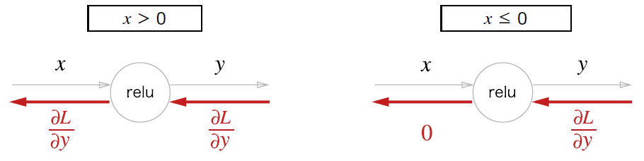
5.5.1 ReLu 계층

ReLU 수식

$x$ 에 대한 $y$ 의 미분

순전파 때의 입력 $x$ 가 0보다 크면 역전파는 상류의 값을 그대로 하류로 보낸다.
순전파 때의 입력 $x$ 가 0 이하면 역전파는 하류로 신호를 보내지 않는다. (0을 보냄)

ReLU 계층 구현

class Relu:
    def __init__(self):
        self.mask = None
 
    def forward(self, x):
        self.mask = (x <= 0)
        out = x.copy()
        out[self.mask] = 0
 
        return out
 
    def backward(self, dout):
        dout[self.mask] = 0
        dx = dout
 
        return dx

ReLU 클래스는 mask라는 인스턴스 변수를 가진다.
mask : True/False로 구성된 넘파이 배열
순전파 입력인 $x$ 원소 값이 0이하면 True, 그 외는 False
역전파 때는 순전파 때 만들어둔 mask를 사용하여 mask의 원소가 True인 곳에서는 상류에서 전파된 dout을 0으로 설정한다.

import numpy as np
 
x = np.array( [[1.0, -0.5], [-2.0, 3.0]])
print(x)
>>> [[ 1.  -0.5]
	[-2.   3. ]]

mask = (x <= 0)
print(mask)
>>> [[False  True]
	[ True False]]

5.6 Affine/Softmax 계층 구현하기

5.6.1 Affine 계층

신경망의 순전파 때 수행하는 행렬의 곱을 기하학에서는 어파인 변환이라고 한다.
따라서 어파인 변환을 수행하는 처리를 'Affine 계층'이라는 이름으로 구현한다.
$Y=np.dot(X,W)+B$ 를 수행한다.

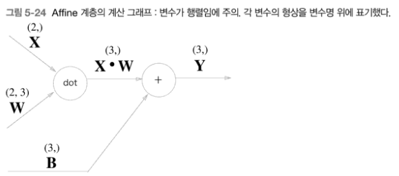
지금까지의 계산 그래프는 노드 사이에 '스칼라값'이 흘렀는 데 반해, 이에서는 '행렬'이 흐르고 있다.
Affine 계층의 역전파를 수식으로 전재하면 다음과 같다.
이때 $W^T$ 의 $T$ 는 전치행렬을 뜻한다.
전치 행렬 : $W$ 의 $(i,j)$ 위치의 원소를 $(j,i)$ 로 바꾼 것을 의미한다.

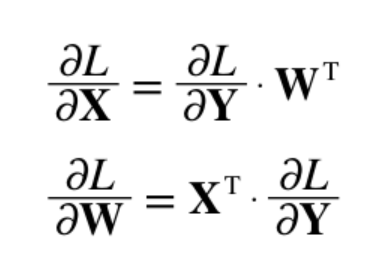
Affine 계층의 역전파를 계산그래프로 나타내면 다음과 같다.
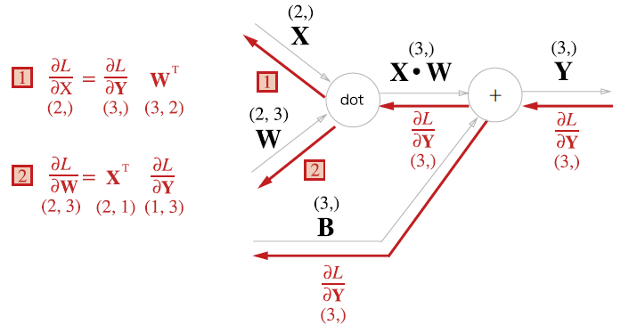
$X$ 와 $\frac{\partial L}{\partial X}$ , $W$ 와 $\frac{\partial L}{\partial W}$ 의 형상이 같다는 것에 주목한다.

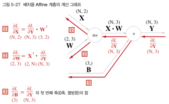
5.6.2 배치용 Affine 계층

앞선 계산 그래프는 하나의 입력 데이터를 고려하였다. 데이터 N개를 묶어 순전파를 전하는 경우, 즉 배치용 Affine 계층을 생각해보자.
기존과 다른 부분은 입력 $X$ 의 형상이 $(N,2)$ 가 된 것이다.
이후로는 지금과 같이 계산 그래프의 순서를 따라 순순히 행렬 연산을 하게 된다.
역전파 때는 행렬의 형상에 주의하면 $\frac{\partial L}{\partial X}$ , $\frac{\partial L}{\partial W}$ 은 이전과 같이 도출할 수 있다.
편향 덧셈 주의 : 순전파 때의 편향 덧셈은 $X*W$ 에 대한 편향이 각 데이터에 더해진다.
ex) N = 2일때, 편향은 그 두 데이터 각각의 계산결과에 더해짐

 
# 순전파 편향 덧셈
X_dot_W = np.array([[0,0,0], [10,10,10]])
B = np.array([1,2,3])
 
print(X_dot_W)
>>> [[ 0  0  0]
	[10 10 10]]
    
print(X_dot_W + B)
>>> [[ 1  2  3]
	[11 12 13]]

순전파의 편향 덧셈이 각각 데이터에 더해지기 때문에, 역전파 때는 각 데이터의 역전파 값이 편향의 원소에 모여야 한다.

dY = np.array([[1,2,3],[4,5,6]])
print(dY)
>>> [[1 2 3]
	[4 5 6]]
    
dB = np.sum(dY, axis=0)
print(dB)
>>> [5 7 9]

예시에서는 데이터가 2개(N=2)라고 가정하였다.
편향의 역전파는 그 두 데이터에 대한 미분을 데이터마다 더해서 구한다.
그래서 np.sum()에서 0번째 축에 대해 (axis=0)의 총합을 구하는 것이다.
상단 이미지를 코드로 구현하면 다음과 같다.

class Affine:
    def __init__(self, W, b):
        self.W = W
        self.b = b
        self.x = None
        self.dW = None
        self.db = None

    def forward(self, x):
        self.x = x
        out = np.dot(self.x, self.W) + self.b

        return out

    def backward(self, dout):
        dx = np.dot(dout, self.W.T)
        self.dW = np.dot(self.x.T, dout)
        self.db = np.sum(dout, axis=0)
        
        return dx

5.6.3 Softmax-with-Loss 계층

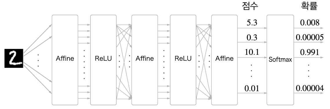
신경망에서 수행하는 작업은 학습과 추론 두 가지이다. 일반적으로 추론일 때는 Softmax 계층(layer)을 사용하지 않는다. Softmax 계층 앞의 Affine 계층의 출력을 점수(score)라고 하는데, 딥러닝의 추론에서는 답을 하나만 예측하는 경우에는 가장 높은 점수만 알면 되므로 Softmax 계층이 필요없다. 반면, 딥러닝을 학습할 때는 Softmax 계층이 필요하다.
손글씨 숫자 인식에서의 Softmax 계층 출력은 다음과 같다.
이와 같이 Softmax 계층은 입력값을 정규화(출력의 합이 1이 되도록 변형)하여 출력한다.
또한 손글씨 숫자는 가짓수가 10개이므로 Softmax 계층의 입력은 10개가 된다.
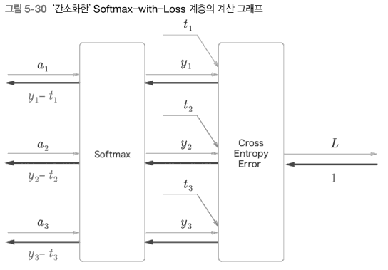
소프트맥스 계층 구현 시, 손실 함수인 교차 엔트로피 오차도 포함하여 'Softmax-with-Loss 계층'이라는 이름으로 구현한다. Softmax-with-Loss 계층의 계산 그래프는 다음과 같다.

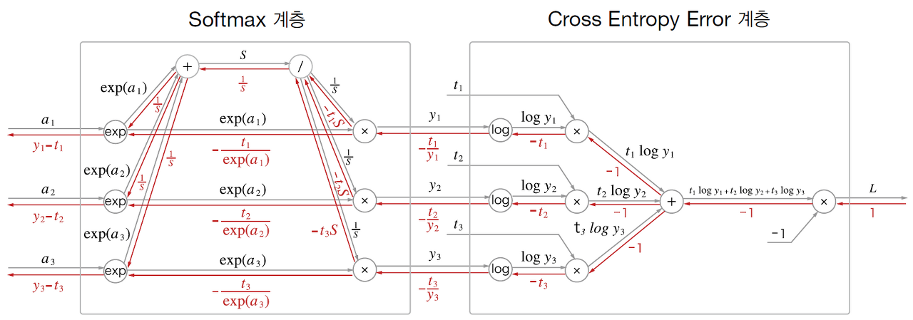
Softmax : 소프트맥스 함수
Cross Entropy Error : 교차 엔트로피 오차
3클래스 분류를가정하고 이전 계층에서 3개의 입력(점수)을 받는다.

[순전파]

Softmax 계층은 입력 $(a_1, a_2, a_3)$ 을 정규화 하여 $(y_1, y_2, y_3)$ 을 출력한다.
Cross Entropy Error 계층은 $(y_1, y_2, y_3)$ 와 정답 테이블 $(t_1, t_2, t_3)$ 을 받고, 이 데이터들로부터 손실 $L$ 을 출력한다.

[역전파]

Softmax 계층의 역전파는 $(y_1-t_1, y_2-t_2, y_3-t_3)$ 라는 결과를 내놓는다.
$(y_1, y_2, y_3)$ 는 Softmax 계층의 출력이고 $(t_1, t_2, t_3)$ 는 정답 레이블이므로, $(y_1-t_1, y_2-t_2, y_3-t_3)$ 는 Softmax 계층의 출력과 정답 레이블의 차분인 셈.
신경망의 역전파에서는 이 차이인 오차가 앞 계층에 전해지는 것이며, 이는 신경망 학습의 중요한 성질이다.
Softmax-with-Loss 계층 구현

class SoftmaxWithLoss:
    def __init__(self):
        self.loss = None # 손실
        self.y = None    # softmax의 출력
        self.t = None    # 정답 레이블(원-핫 벡터)
        
    def forward(self, x, t):
        self.t = t
        self.y = softmax(x)
        self.loss = cross_entropy_error(self.y, self.t)
        return self.loss

    def backward(self, dout=1):
        batch_size = self.t.shape[0]
        if self.t.size == self.y.size:
        
        return dx

kimgaeul02

이전 포스트

[프로그래머스] 정렬 - H-Index(Python3)

다음 포스트