[머신러닝] 하이퍼파라미터 튜닝 (Hyperparameter Tuning) - Bayesian Optimization을 이용한 HyperOpt / Optuna

• ✔ HyperOpt

  HyperOpt는 이전 포스팅에서 설명한 Bayesian Optimization의 접근 방식을 취한다. 그럼, HyperOpt를 이용한 Hyperparameter Tuning 과정을 실습을 통해 알아보겠다.
  
  

  • HyperOpt 설치

    먼저, HyperOpt를 설치해보겠다. 다음의 명령어로 설치할 수 있다.

    pip install hyperopt

  • 실습을 위한 데이터 로드

    실습을 위해 Boston 주택 가격 데이터를 로드하였다.

from sklearn.datasets import load_boston
from sklearn.model_selection import train_test_split

# load dataset
data = load_boston()

# train, test split
x_train, x_test, y_train, y_test = train_test_split(data['data'], data['target'], random_state=1)

print(x_train.shape, y_train.shape)
# 출력
# (379, 13) (379,)

• 평가 함수 정의 (RMSE)

  모델의 평가 함수를 정의함. Regression 예측을 하기에, RMSE를 평가 지표로 사용

from sklearn.metrics import mean_squared_error

def RMSE(y_true, y_pred):
    return np.sqrt(mean_squared_error(y_true, y_pred))

• HyperOpt를 활용한 XGBoost 튜닝 예제

  space 변수에는 dictionary 생성 후 hyperparameter 이름을 key, hyperparameter 범위를 value로 지정해 줄 수 있다.

  • hp.choice (hyperparameter 이름, 범위) : 범위 안에 존재하는 값 중 하나를 선택하여 대입하면서 최적의 hyperparameter를 찾음

  • hp.quniform (hyperparameter 이름, start, end, step) : start ~ end 까지 step 간격으로 생성된 후보군 중 최적의 hyperparameter를 찾음

  • hp.uniform (hyperparameter 이름, start, end) : start ~ end 사이의 임의의 값 중 최적의 hyperparameter를 찾음

import hyperopt
from hyperopt import fmin, tpe, hp, STATUS_OK, Trials
from sklearn.metrics import mean_squared_error

# regularization candiate 정의
reg_candidate = [1e-5, 1e-4, 1e-3, 1e-2, 0.1, 1, 5, 10, 100]

# space 정의, Hyperparameter의 이름을 key 값으로 입력
space={'max_depth': hp.quniform("max_depth", 5, 15, 1),
       'learning_rate': hp.quniform ('learning_rate', 0.01, 0.05, 0.005),
       'reg_alpha' : hp.choice('reg_alpha', reg_candidate),
       'reg_lambda' : hp.choice('reg_lambda', reg_candidate),
       'subsample': hp.quniform('subsample', 0.6, 1, 0.05),
       'colsample_bytree' : hp.quniform('colsample_bytree', 0.6, 1, 0.05),
       'min_child_weight' : hp.quniform('min_child_weight', 1, 10, 1),
       'n_estimators': hp.quniform('n_estimators', 200, 1500, 100)
      }

# 목적 함수 정의
# n_estimators, max_depth와 같은 반드시 int 타입을 가져야 하는 hyperparamter는 int로 타입 캐스팅 합니다.
def objective(space):
    model=XGBRegressor(n_estimators =int(space['n_estimators']), 
                       max_depth = int(space['max_depth']), 
                       learning_rate = space['learning_rate'],
                       reg_alpha = space['reg_alpha'],
                       reg_lambda = space['reg_lambda'],
                       subsample = space['subsample'],
                       colsample_bytree = space['colsample_bytree'], 
                       min_child_weight = int(space['min_child_weight']))
    
    evaluation = [(x_train, y_train), (x_test, y_test)]
    
    model.fit(x_train, y_train,
              eval_set=evaluation, 
              eval_metric="rmse",
              early_stopping_rounds=20,
              verbose=0)

    pred = model.predict(x_test)
    rmse= RMSE(y_test, pred)    
    # 평가 방식 선정
    return {'loss':rmse, 'status': STATUS_OK, 'model': model}

random_state 인자는 Bayesian Optimization 상의 랜덤성이 존재하는 부분(e.g. 다음 입력값 후보 추출 등)을 통제할 수 있도록 random seed를 입력해 주기 위한 목적으로 입력된다. 랜덤성을 통제할 필요가 없을 경우 입력하지 않아도 무방하다.

위와 같이 목적 함수가 정의가 완료되었으면, fmin 함수로 최적화를 지정해준다.
fmin에는 다양한 옵션 값을 지정할 수 있다.

# Trials 객체 선언합니다.
trials = Trials()
# best에 최적의 하이퍼 파라미터를 return 받습니다.
best = fmin(fn=objective,
            space=space,
            algo=tpe.suggest,
            max_evals=50, # 최대 반복 횟수를 지정합니다.
            trials=trials)

# 최적의 Hyperparameter 조합
print (best)

{'colsample_bytree': 0.9500000000000001,
'learning_rate': 0.01,
'max_depth': 6,
'min_child_weight': 1,
'n_estimators': 600,
'reg_alpha': 1e-05,
'reg_lambda': 0.01,
'subsample': 0.75}

best를 통해 최적의 조합이 도출되었으니, 이를 바탕으로 모델을 학습시켜야 한다. 다만, best는 hp.choice를 쓸 때, index 값으로 추출을 해준다. 따라서, 이를 인덱싱을 통해 다시 원래의 값으로 변환해주어야 한다.
hp.uniform, hp.quniform 으로 추출한 것은 그대로 사용하면 된다. 다만, float 형식으로 나오기 때문에, 이를 int 형식으로 바꿔주면 된다.

best['max_depth'] = int(best['max_depth'])
best['min_child_weight'] = int(best['min_child_weight'])
best['n_estimators'] = int(best['n_estimators'])
best['reg_alpha'] = reg_candidate[int(best['reg_alpha'])]
best['reg_lambda'] = reg_candidate[int(best['reg_lambda'])]


xgb = XGBRegressor(**best)
xgb.fit(x_train, y_train)
pred = xgb.predict(x_test)
print(RMSE(y_test, pred))

2.7264573146141746

• ✔ Optuna

  • Hyperparameter Tuning 에 쓰이고 있는 최신 AutoML 기법
  • 간단하고 빠르게 튜닝이 가능
  • 간단한 메소드로 시각화 가능
  • 거의 모든 ML/DL 프레임워크에서 사용 가능한 넓은 범용성을 지님
  • 아래의 예시를 통해 더 자세하게 알아보자.

  import optuna
  from optuna import Trial, visualization
  from optuna.samplers import TPESampler
  
  from sklearn.metrics import mean_absolute_error

  • trial.suggest_int : 범위 내의 정수형 값을 선택함
    trial.suggest_int('n_estimators', 100, 500)

  • trial.suggest_categorical : list 내의 데이터 중 선택함 trial.suggest_categorical('criterion', ['gini', 'entropy'])

  • trial.suggest_uniform : 범위 내의 이산 균등 분포를 값으로 선택함
    trial.suggest_uniform('subsample', 0.2, 0.8)

  • trial.suggest_discrete_uniform : 범위 내의 이산 균등 분포를 값으로 선택 trial.suggest_discrete_uniform('max_features', 0.05, 1, 0.05)

  • trial.suggest_loguniform : 범위 내의 로그 함수 선상의 값을 선택함
    trial.suggest_loguniform('learning_rate' : 1e-6, 1e-3)

# 목적 함수 지정
# XGB 하이퍼 파라미터들 값 지정
def objectiveXGB(trial: Trial, X, y, test):
    param = {
        'n_estimators' : trial.suggest_int('n_estimators', 500, 4000),
        'max_depth' : trial.suggest_int('max_depth', 8, 16),
        'min_child_weight' : trial.suggest_int('min_child_weight', 1, 300),
        'gamma' : trial.suggest_int('gamma', 1, 3),
        'learning_rate' : 0.01,
        'colsample_bytree' : trial.suggest_discrete_uniform('colsample_bytree', 0.5, 1, 0.1),
        'nthread' : -1,
        # 'tree_method' : 'gpu_hist',
        # 'predictor' : 'gpu_predictor',
        'lambda' : trial.suggest_loguniform('lambda', 1e-3, 10.0),
        'alpha' : trial.suggest_loguniform('alpha', 1e-3, 10.0),
        'subsample' : trial.suggest_categorical('subsample', [0.6,0.7,0.8,1.0]),
        'random_state' : 1
    }
    
    # 학습 모델 생성
    model = XGBRegressor(**param)
    xgb_model = model.fit(X, y, verbose=True)
    
    # 모델 성능 확인
    score = mean_absolute_error(xgb_model.predict(X), y)
    
    return score

# direction : score 값을 최대 or 최소로 하는 방향으로 지정 (minimize or maximize)
study = optuna.create_study(direction='minimize', sampler=TPESampler())

# n_trials : 시도 횟수 (미 입력 시 무한 반복, 따라서 필수 기입)
study.optimize(lambda trial : objectiveXGB(trial, X, y, X_test), n_trials = 50)

print('Best trial : score {}, \nparams : {}'.format(study.best_trial.value, study.best_trial.params))

Best trial : score 0.6918131483269861,
params : {'n_estimators': 1988, 'max_depth': 15, 'min_child_weight': 171, 'gamma': 2, 'colsample_bytree': 0.7, 'lambda': 0.009025835256777458, 'alpha': 1.0684343216052703, 'subsample': 0.6}

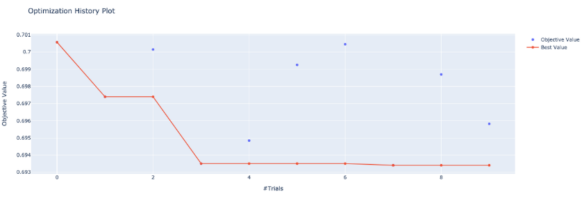
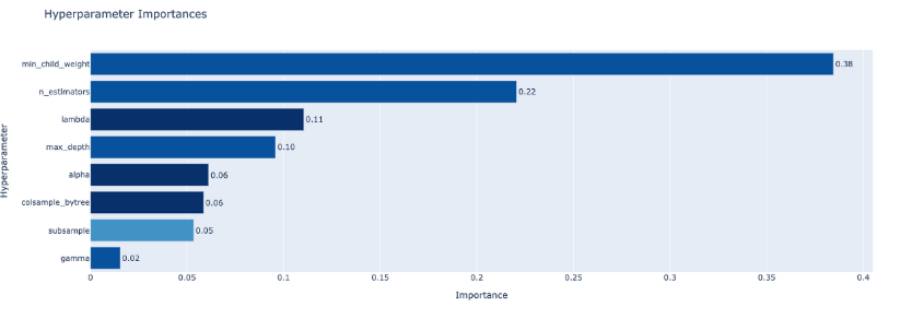
optuna는 학습하는 절차를 확인할 수 있는 시각화 툴도 제공한다. 다양한 시각화 기법을 제공하지만, hyperparameter 별 중요도를 확인할 수 있는 함수와, 매 trial 마다 Loss가 어떻게 변화하였는지 확인할 수 있는 함수를 확인해보겠다. (아래 그림은 단순 예시이다.)

optuna.visualization.plot_param_importances(study) # 파라미터 중요도 확인 그래프

optuna.visualization.plot_optimization_history(study) # 최적화 과정 시각화